ayeimanolr

Modelling – mixed effects – concepts

Posted on May 15, 2013 by robayedavies

I am going to take another shot at considering mixed effects modelling. This time from a perspective closer to my starting point. I first learnt about mixed-effects modelling through reading about it in, I think, some paper or chapter by Harald Baayen in the mid-2000s (maybe, Baayen et al., 2002). In 2007, I attended a seminar by Marc Brysbaert on ‘The Language as fixed-effect fallacy’ which ended in a recommendation to consider mixed-effects modelling and to try lmer in R. The workshop title is a reference to a highly influential paper by Clark (1973; see, also, Raaijmakers et al., 1999) and a familiar problem for many psycholinguists.

The problem is this:

Creative commons – flickr – National Media Museum: ‘Fear’ from ‘The Expression of Emotions in Man and Animals’ London 1872. Charles Darwin (1809-1882)

I might have an expectation about some language behaviour, for example, that words appearing often in the language are easier to read, or that word choice in speaking is mediated through a process of selection by competition. I perform an experiment in which I test some number of individuals (let’s say, 20) with some number of stimuli (let’s say 20). Perhaps the stimuli vary in frequency, or perhaps I present them in two conditions (say, once superimposed on pictures of semantically related objects, once on pictures of unrelated objects). I do not really care who any one person is, I am mostly interested in the effect of frequency or semantic relatedness in general, and regard the specific characteristics of the people being tested as random variation, seeing the group of people being tested as a random sample from the population of readers or speakers. Likewise, I wish to infer something about language and would consider the particular words being presented as a random sample from the wider population of words. For both samples, I would wish to estimate the effect of interest to me while accounting for random variation in performance due to participant or item sampling.

Clark (1973) argued that to draw conclusions from data like these that might apply generally, one ought to analyze the data using an approach that took into account the random effects of both participants and individuals. As I noted previously, if you look at data on a participant-by-participant basis, you will find ample evidence for both variation across individuals about some average effect and variation across items about some average effect.

Individual differences – adults reading aloud, 100 words, English – RT by log frequency

Around 2006, I was conducting a regression analysis of Spanish reading data and finding quite big variation in the size and sometimes the direction of effects across individuals all of whom had been presented with the same words under the same circumstances.

Now, if you look at Clark’s (1973) paper, you can see him consider what researchers at the time did and what they should do about subject and item random effects. Conventionally, one had averaged across responses to the different words for each participant to get an average RT by-subjects per condition, ignoring variation between items (the fact that the items were sampled from a wider population) and thus inflating the possibility that an effect is spuriously detected when it is not present. The key difficulty is to estimate error variance appropriately. One is seeking to establish if variance due to an effect is greater than variance due to error variation, but this will only guide us correctly if the error variance includes both error variance due to subject and that due to item sampling. Clark (1973) recommended calculating F’, the quasi F-ratio, as the ratio of the variance due to the effect compared to the variance due to variance (in the effect) due to random variation between subjects or items. As a shortcut to the needed analysis, Clark (1973) suggested one could perform an analysis of the effect as it varied by subjects and an analysis of the effect as it varied by items. Conventionally, this subsequently meant that one could average over responses to different items for each person to get the average responses by-subjects and perform a by-subjects ANOVA (F1) or t-test (t1), and one could also average over responses by different people to each item to get the average responses by-items and perform a by-items ANOVA (F2) or t-test (t2). Using a very simple formula, one could then form minF’ as the ratio:

$\frac{F_1F_2}{F_1 + F_2}$

and then more accurately estimate the effect with respect to the null hypothesis taking into account both subject and item random effects.

Not simple enough, as Raaijmakers et al. (1999) report, psychologists soon stopped calculating minF’ and resorted just to reporting F1 and F2 separately or (informally) together. It has been quite typical to refer to an effect that is significant in F1 and F2 as significant but Raaijmakers et al. (1999) show that even if F1 + F2 are significant that does not mean that minF’ will be.

I spent a bit of time calculating minF’ and, if I were doing ANOVA and not lmer, I would do it still (see Baayen et al., 2008, for an analysis of how well minF’ does in terms of both Type I and II errors).

That is fine. But what if you’re doing a reading experiment in which you are concerned about the effects on reading of item attributes and you have read Cohen (1983) or his other commentary on the cost of dichotomizing continous variables? What you would not do is present items selected to conform to the manipulation of some factor e.g. selecting items that were low in frequency or high in frequency (but matched on everything else) to test the effect of frequency on reading. This is because in performing a factorial study like that, essentially, cutting a continuous variable (like frequency) into two, one is reducing the capacity of the analysis to detect an effect that really is there (increasing the Type II error rate), as Cohen (1983) explained. What you would do, then, is to perform a regression analysis. In most circumstances, one might present a large-ish set of words to a sample of participants, giving each person the same words so that the study take a repeated-measures approach. One can then average over subjects for each word to get the average by-items reaction times (or proportion of responses correct) and then perform an analysis of the manner in which reading performance is affected by an item attribute like frequency.

However, Lorch & Myer (1990) pointed out that if you performed by-items regressions on repeated measures data then you would be vulnerable to the effect of making subjects a fixed effect: effects might be found to be significant simply because of variation over subjects in the effect of the item attribute. They recommend a few alternatives. One is to not average data over subjects but arrange the raw observations (one RT corresponding to a person’s response to a word) in a long format database then perform a regression in which: 1. item attributes are predictors (in long format, one would have to copy item attribute data for each person’s observations); 2. subject identity is coded using dummy coding variables (with n subjects – 1 columns). Another approach is to perform a regression analysis for each person’s data individually, then conduct a further test (e.g. a one-sample t-test) of whether a vector of the per-person regression coefficients for an effect is significantly different from zero. Balota et al. (2004) take the latter approach.

But you can see the potential problems if you look at the lattice of individual data plots above, and at the following plot from an old study of mine:

60 children, aged 10-12 years, logRT reading aloud by logcelex frequency

What you can see is the effect of frequency on the performance of each individual reader, estimated in a per-individual regression analysis.

Notice:

— Variation in the intercept i.e. the average RT per person.

— Variation in the slope of the effect.

If you think about it, and look at some of the low-scoring participants in the lattice plot, above, you can also see that the size of the sample of observations available for each person will also vary. Doing a t-test on effects coefficients calculated for each individual will not allow you to take into account the variation in reliability of that effect over the sample.

As Baayen et al. (2008) point out, it turns out that both the by-items regressions and by-subjects regression approaches have problems accounting properly for random effects due to subjects and to items (with departures from the nominal error rate i.e. p does not necessarily = 0.05 when these analyses say it does), and may suffer from restricted sensitivity to effects that really are present.

It is at that point, that I turned to mixed-effects modelling.

Reading

Baayen, R. H., Davidson, D. J., & Bates, D. M. (2008). Mixed-effects modeling with crossed random effects for subjects and items. Journal of Memory and Language, 59, 390-412.
Baayen, R. H., Tweedie, F. J., & Schreuder, R. (2002). The subjects as a simple random effect fallacy: Subject variability and morphological family effects in the mental lexicon. Brain and Language, 81, 55-65.
Balota, D., Cortese, M. J., Sergent-Marshall, S. D., Spieler, D., & Yap, M. (2004). Visual word recognition of single-syllable words. Journal of Experimental Psychology: General, 133, 283-316.
Brysbaert, M. (2008). “The language-as-fixed-effect fallacy”: Some simple SPSS solutions to a complex problem.
Clark, H. H. (1973). The language-as-fixed-effect fallacy: A critique of language statistics in psychological science. Journal of Verbal Learning and Verbal Behaviour, 12, 335-359.
Cohen, J. (1983). The cost of dichotomization. Applied Psychological Measurement, 7, 249-253.
Lorch, R. F., & Myers, J. L. (1990). Regression Analyses of Repeated Measures Data in Cognitive Research. Journal of Experimental Psychology: Learning, Memory and Cognition, 16(1), 149-157.
Raaijmakers, J. G. W., Schrijnemakers, J. M. C., & Gremmen, F. (1999). How to deal with the “Language-as-fixed-effect Fallacy”: Common misconceptions and alternative solutions. Journal of Memory and Language, 41, 416-426.

Posted in 16. Modelling - mixed-effects | Tagged anova(), F', lmer(), minF', mixed effects, mixed-e, regression | Leave a comment

Picture break

Posted on May 14, 2013 by robayedavies

Picture taken in San Francisco flower conservatory, a wonderful place with wonderfully informative guides.

We will go on to a bit more model checking before considering the random effects formally.

Posted in .Interim directions | Leave a comment

Mixed effects – continuing the extended example

Posted on May 14, 2013 by robayedavies

As noted in a previous post, our mixed effects analysis of the ML lexical decision data suggested that RTs were influenced by significant effects due to:

cAge + cART + cTOWRENW +

cLength + cOLD + cBG_Mean + cLgSUBTLCD + cIMG +

cTOWRENW:cLgSUBTLCD + cAge:cLength + cAge:cOLD + cAge:cBG_Mean

I am writing the interactions not as var1*var2 but as var1:var2 – the second form of expressing an interaction restricts the analysis to considering just that product term.

I have been advised to check whether such effects are dependent in some way on the presence of other, nonsignificant effects (I think this recommendation might be in Baayen, 2008, but I know it has come to me also through other channels). That check can take the form of a re-analysis of the data with a model (REML = FALSE) including just the significant effects from the first analysis.

For our situation, the code for doing that model would be written as follows:


# we can check if the significant effects are influenced by the presence of nonsig effects by rerunning the model
# first removing all but the significant effects

full.lmer5 <- lmer(log(RT) ~

 cAge + cART + cTOWRENW +

 cLength + cOLD + cBG_Mean + cLgSUBTLCD + cIMG +

 cTOWRENW:cLgSUBTLCD + cAge:cLength + cAge:cOLD + cAge:cBG_Mean +

 (1|subjectID) + (1|item_name),

 data = nomissing.full, REML = FALSE)

print(full.lmer5,corr=F)
pvals.fnc(full.lmer5)$fixed

And, in fact, you can see that some effects that were significant do not remain so once you take out all the effects that were not significant in the previous, full, model.

Notice:

— The effects of age, length, frequency, imageability, the interaction between the nonword reading skill and the frequency effects, and between the age and orthographic OLD effect, remain significant while the others are rendered either nonsignificant or marginal.

— We included main effects even if not originally significant, if they had been part of a significant interaction: the interaction is what counts but the main effect (to use the ANOVA term) has to be in the model for it to be properly specified.

I would also note that some authors do not recommend the removal of nonsignificant effects (e.g. Harrell, 2001) and I think that that would be my inclination also. I have found that the significance of some effects – the flakier, or more delicate, and also often the effects of most interest – may move around depending on what else is also specified for the model. That is what you might call a pragmatic emotional concern – the instability is worrisome – but this is an instability that also reflects the impact on effect of estimation of modifications in the predictor space. We could argue that the model should be the most complex that can be found to be justified.

What have we learnt

(The code used to run this analysis can be found here.)

That some effects might be dependent on the presence of other non-significant effects.

Note the key vocabulary in the use of X:Y rather than X*Y interaction notation; see Baayen (2008) for further explanation.

Reading

Baayen, R. H. (2008). Analyzing linguistic data: Cambridge University Press.
Harrell Jr, F. J. (2001). Regression modelling strategies: With applications to linear models, logistic regression, survival analysis. New york, NY: Springer.
Snijders, T.A.B., & Bosker, R.J. (2004). Multilevel analysis: An introduction to basic and advanced multilevel modeling. London: Sage Publications Ltd.

Posted in 16. Modelling - mixed-effects | Tagged lmer(), mixed effects | Leave a comment

Modelling – mixed effects – concepts

Posted on May 14, 2013 by robayedavies

In the previous post, we ran through an extended example of a mixed-effects modelling analysis of the ML lexical decision data. We ended the post by getting p-values for the effects of the predictors included in our model. That was the model apparently justified by a likelihood ratio test comparison of maximum likelihood (REML=F) models varying in fixed effects but constant in possessing random effects of subjects and items on intercepts.

You will recall that I said in that post that:

In following posts, we shall 1. perform some checks on whether the fixed effects appear justified with respect to data hygiene 2. examine what random effects seem justified, looking at random effects on intercepts and random effects on slopes.

— that will happen but I want to consider some of the words I am using.

Creative commons – flickr – Florida Memory: Fisherman with his son, Naples, Florida, 1949

I am reading the great introductory text on multilevel modeling by Snijders & Boskers (2004). There, they begin their book with a clear, simple, explanation of the normal data collection situation for many of us.

You will know that statistical models, for example, ordinary least squares (OLS) regression assume that observations should be sampled independently. In regression, the distribution of errors – the differences between model prediction and data observation for any observation – should consist of errors with a normal distribution, with any one error independent of any other. If we think about the normal situation in which we find ourselves, that independence assumption will be invalid. Most of the time, we are asking participants to read some set of words, and everyone will be asked to read all the words. If you plot the participants’ data or the responses to each item, you will see that, as you might expect, some people are slow and some fast for most responses to most words, while some words are easy and some hard for most people.

You can consider this illustration of some reading data, as an illustration of that point.

Notice:

— Each participant in this study of reading aloud was an adult and each was asked to read the same set of about 100 words out loud.

— The lattice of plots shows:

1. The average RT for each person – and for each word – varied. You might guess what the average over all people or all words would be. Now consider how each person’s average RT varies from the average RT over all people, or how each word’s average RT varies from the average RT over all words. The average outcome is called the intercept, a term you will have encountered before in regression. Estimating the deviation of a person or a word from the overall average is a matter of estimating random effects on person or word on intercepts, or, random intercepts. In the mixed effects modeling code in R, we designate this as:

$(1|subject) + (1|item)$

2. The slope of the effect of, here, frequency on reading RT also appears to vary between people. There might be an average effect of frequency on RT overall. You could call the frequency effect the fixed effect here. We can see that, most of the time, more frequent words are associated with shorter RTs. However, the slope of that effect is more or less steep for some people. That variation in slope can be estimated as random effects of person on slopes, or random slopes. However, the variation in the frequency effect might also be considered to be of theoretical interest and, critically, it might be captured by, for example, an interaction between the effect of frequency and the effect of some participant attribute that conditions or modulates the frequency effect by a systematic (rather than a random) person effect.

Let’s return to Snijders & Boskers (2004). They note that one can often, for reasons of efficiency (consider how much easier it is to give everybody the same sample of words than different samples) or other pragmatic considerations, that data collection often proceeds through multistage sampling. One might test in a set of schools, a sample of schools, and in those schools test samples of children. It is a mistake to consider that the children are sampled independently (an assumption you would be making if you applied OLS regression to such data). That is because the children are clearly grouped by school (and thus not independent samples). Similarly, it would be clearly a mistake to consider that the observations for each person or each word are somehow independent. They are dependent because the data can be considered to cluster or group by person or by word. The consequence of ignoring this structure will be inflated Type I error rate, or finding things that are not really there.

Snijders & Boskers (2009) next point out, however, that if data are collected in multistage sampling we might, for theoretical or practical reasons, want to make inferences about effects occurring at each stage. (This is also noted by Baayen, Davidson & Bates (2008) in comments that led me to consider how the effects of item attributes might vary between readers systematically rather than merely at random.) We might want to know how school environment or policy affects teacher practice or how both school policy and teacher attitudes affect student performance. We might want to know how the kind of reader you are affects reading performance but also how the kind of word you read affects performance. We might, further, be interested in how effects that operate at one level or over one kind of cluster interact with effects operating at other levels or over other kinds of cluster.

The more that observations within a cluster are similar to each other (compared to other clusters) the more we might be concerned about the characteristics of the cluster, the higher level units.

We must not forget longitudinal observations, and shall return to the situation where data are clustered because people are tested repeatedly over time.

Reading

Snijders, T.A.B., & Bosker, R.J. (2004). Multilevel analysis: An introduction to basic and advanced multilevel modeling. London: Sage Publications Ltd.

Posted in 16. Modelling - mixed-effects | Tagged hierarchical, mixed effects, multilevel | Leave a comment

Modelling – extended example mixed-effects analysis

Posted on May 12, 2013 by robayedavies

In the previous post, we ran through an example of a mixed-effects analysis completed using the lmer() function from the lme4 package (Bates, 2005; Bates, Maelchler & Bolker, 2013).

We will not, yet, really fulfill the promise to develop our understanding but we will add snippets of vocabulary for the area that we shall return to later.

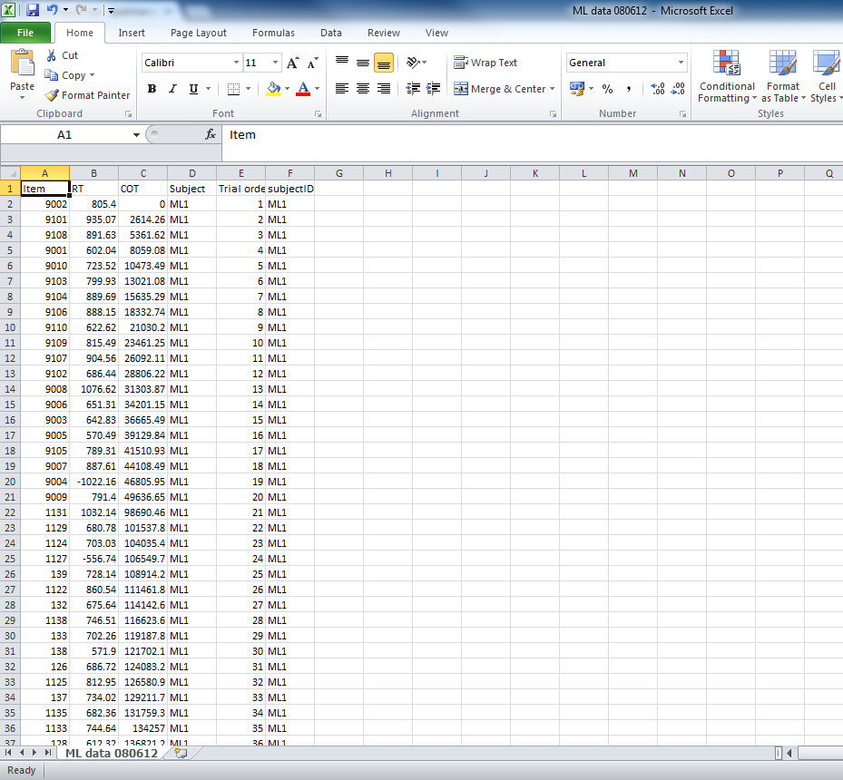
We are working, again, with the dataframe collated in previous posts (see here), which combines data about subject attributes, item attributes, and the observed behavioural responses (keypress responses in lexical decision) of the participants to a set of 160 words.

In this post, we will consider a more extended example. We will work through a series of models in a sequence to examine what fixed effects appear to improve the capacity of the model to fit the observed responses.

In following posts, we shall 1. perform some checks on whether the fixed effects appear justified with respect to data hygiene 2. examine what random effects seem justified, looking at random effects on intercepts and random effects on slopes.

We shall also consider how to produce partial effects plots depicting the effects i.e. the model predictions taking everything into account.

Note the terms in use in this area. People (e.g. Pinheiro & Bates, 2000) often refer to fixed effects as the effects on response variance due to variables that are manipulated (e.g. different conditions) or where variation can be replicated (e.g. presenting long vs. short words). They then refer to random effects as the effects on response variance corresponding to grouping units (e.g. subjects who all read some set of words) in sampling. Pinheiro & Bates (2000) explain that a mixed-effects model has both fixed effects and random effects. Some authors (e.g. Gelman & Hill, 2007) assert, as I understand it, that the distinction tends to break down if you put the idea under pressure.

As usual, we will work through a series of self-annotated phases.

Load libraries, define functions, load data

We start by loading the libraries of functions we are likely to need, defining a set of functions not in libraries, setting the working directory, and loading the dataframe we will work with into the R session workspace.


# load libraries of packages #############################################################################
library(languageR)
library(lme4)
library(ggplot2)
library(grid)
library(rms)
library(plyr)
library(reshape2)
library(psych)
library(gridExtra)

&nbsp;

# define functions #######################################################################################
# pairs plot function

#code taken from part of a short guide to R
#Version of November 26, 2004
#William Revelle
# see: http://www.personality-project.org/r/r.graphics.html

panel.cor <- function(x, y, digits=2, prefix="", cex.cor)
{
 usr <- par("usr"); on.exit(par(usr))
 par(usr = c(0, 1, 0, 1))
 r = (cor(x, y))
 txt <- format(c(r, 0.123456789), digits=digits)[1]
 txt <- paste(prefix, txt, sep="")
 if(missing(cex.cor)) cex <- 0.8/strwidth(txt)
 text(0.5, 0.5, txt, cex = cex * abs(r))
}
# just a correlation table, taken from here:
# http://myowelt.blogspot.com/2008/04/beautiful-correlation-tables-in-r.html
# actually adapted from prvious nabble thread:

corstarsl <- function(x){
 require(Hmisc)
 x <- as.matrix(x)
 R <- rcorr(x)$r
 p <- rcorr(x)$P

 ## define notions for significance levels; spacing is important.
 mystars <- ifelse(p < .001, "***", ifelse(p < .01, "** ", ifelse(p < .05, "* ", " ")))

 ## trunctuate the matrix that holds the correlations to two decimal
 R <- format(round(cbind(rep(-1.11, ncol(x)), R), 2))[,-1]

 ## build a new matrix that includes the correlations with their apropriate stars
 Rnew <- matrix(paste(R, mystars, sep=""), ncol=ncol(x))
 diag(Rnew) <- paste(diag(R), " ", sep="")
 rownames(Rnew) <- colnames(x)
 colnames(Rnew) <- paste(colnames(x), "", sep="")

 ## remove upper triangle
 Rnew <- as.matrix(Rnew)
 Rnew[upper.tri(Rnew, diag = TRUE)] <- ""
 Rnew <- as.data.frame(Rnew)

 ## remove last column and return the matrix (which is now a data frame)
 Rnew <- cbind(Rnew[1:length(Rnew)-1])
 return(Rnew)
}

&nbsp;

# read in data files #####################################################################################

getwd()
# set the working directory

setwd("C:/Users/p0075152/Dropbox/resources R public")

# read in the full database

RTs.norms.subjects <- read.csv("RTs.norms.subjects 090513.csv", header=T, na.strings = "-999")

If you run all that code, you will see the dataframes and functions appear listed in the workspace window of R-studio.

Prepare data – remove errors

As in the previous post, we need to remove errors from the dataframe. We can do this by setting a condition on rows, subsetting the dataframe to a new dataframe where no RT is less than zero because DMDX outputs .azk datafiles in which incorrect RTs are listed as negative numbers.


# preparing our dataframe for modelling ##################################################################
# the summary shows us that there are negative RTs, which we can remove by subsetting the dataframe
# by setting a condition on rows

nomissing.full <- RTs.norms.subjects[RTs.norms.subjects$RT > 0,]

# inspect the results

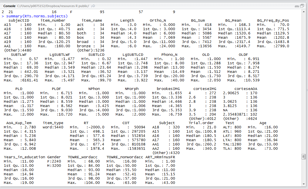
summary(nomissing.full)

# how many errors were logged?

# the number of observations in the full database i.e. errors and correct responses is:

length(RTs.norms.subjects$RT)

# > length(RTs.norms.subjects$RT)
# [1] 5440

# the number of observations in the no-errors database is:

length(nomissing.full$RT)

# so the number of errors is:

length(RTs.norms.subjects$RT) - length(nomissing.full$RT)

# > length(RTs.norms.subjects$RT) - length(nomissing.full$RT)
# [1] 183

# is this enough to conduct an analysis of response accuracy? we can have a look but first we will need to create
# an accuracy coding variable i.e. where error = 0 and correct = 1

RTs.norms.subjects$accuracy <- as.integer(ifelse(RTs.norms.subjects$RT > 0, "1", "0"))

# we can create the accuracy variable, and run the glmm but, as we will see, we will get an error message, false
# convergence likely due to the low number of errors

Notice:

— I am copying the outputs from function calls from the console window, where they appear, into the script file, where they are now saved for later reference.

— I find this to be a handy way to keep track of results, as I move through a series of analyses. This is because I often do analyses a number of times, maybe having made changes in the composition of the dataframe or in how I transformed variables, and I need to keep track of what happens after each stage or each operation.

— You can see that there were a very small number of errors recorded in the experiment, less than 200 errors out of 5000+ trials. This is a not unusual error rate, I think, for a dataset collected with typically developing adult readers.

In this post, I will add something new, using the ifelse() control structure to create an accuracy variable which is added to the dataframe:


# so the number of errors is:

length(RTs.norms.subjects$RT) - length(nomissing.full$RT)

# > length(RTs.norms.subjects$RT) - length(nomissing.full$RT)
# [1] 183

# is this enough to conduct an analysis of response accuracy? we can have a look but first we will need to create
# an accuracy coding variable i.e. where error = 0 and correct = 1

RTs.norms.subjects$accuracy <- as.integer(ifelse(RTs.norms.subjects$RT > 0, "1", "0"))

# we can create the accuracy variable, and run the glmm but, as we will see, we will get an error message, false
# convergence likely due to the low number of errors

Notice:

— I am starting to use the script file not just to hold lines of code to perform the analysis, not just to hold the results of analyses that I might redo, but also to comment on what I am seeing as I work.

— The ifelse() function is pretty handy, and I have started using it more and more.

— Here, I can break down what is happening step by step:-

1. RTs.norms.subjects$accuracy <- — creates a vector that gets added to the existing dataframe columns, that vector has elements corresponding to the results of a test on each observation in the RT column, a test applied using the ifelse() function, a test that results in a new vector with elements in the correct order for each observation.

2. as.integer() — wraps the ifelse() function in a function call that renders the output of ifelse() as a numeric integer vector; you will remember from a previous post how one can use is.[datatype]() and as.[datatype]() function calls to test or coerce, respectively, the datatype of a vector.

3. ifelse(RTs.norms.subjects$RT > 0, “1”, “0”) — uses the ifelse() function to perform a test on the RT vector such that if it is true that the RT value is greater than 0 then a 1 is returned, if it is not then a 0 is returned, these 1s and 0s encode accuracy and fill up the new vector being created, one element at a time, in an order corresponding to the order in which the RTs are listed.

I used to write notes on my analyses on paper, then in a word document (using CTRL-F that will be more searchable), to ensure I had a record of what I did.

It is worth keeping good notes on what you do because you (I) rarely get an unbroken interval of time in which to complete an analysis up to the report stage, thus you will often return to an analysis after a break of days to months, and you will therefore need to write notes that your future self will read so that analyses are self-explanatory or self-explained.

Check predictor collinearity

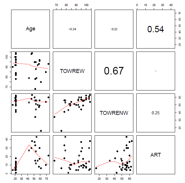
The next thing we want to do is to examine the extent to which our predictors cluster, representing overlapping information, and presenting potential problems for our analysis. We can do this stage of our analysis by examining scatterplot matrices and calculating the condition number for our predictors. Note that I am going to be fairly lax here, by deciding in advance that I will use some predictors but not others in the analysis to come. (If I were being strict, I would have to find and explain theory-led and data-led reasons for including the predictors that I do include.)


# check collinearity and check data distributions #########################################################
# we can consider the way in which potential predictor variables cluster together

summary(nomissing.full)

# create a subset of the dataframe holding just the potential numeric predictors
# NB I am not bothering, here, to include all variables, e.g. multiple measures of the same dimension

nomissing.full.pairs <- subset(nomissing.full, select = c(

 "Length", "OLD", "BG_Mean", "LgSUBTLCD", "brookesIMG", "AoA_Kup_lem", "Age",
 "TOWRE_wordacc", "TOWRE_nonwordacc", "ART_HRminusFR"

 ))

# rename those variables that need it for improved legibility

nomissing.full.pairs <- rename(nomissing.full.pairs, c(

 brookesIMG = "IMG", AoA_Kup_lem = "AOA",

 TOWRE_wordacc = "TOWREW", TOWRE_nonwordacc = "TOWRENW", ART_HRminusFR = "ART"

 ))

# subset the predictors again by items and person level attributes to make the plotting more sensible

nomissing.full.pairs.items <- subset(nomissing.full.pairs, select = c(

 "Length", "OLD", "BG_Mean", "LgSUBTLCD", "IMG", "AOA"

))

nomissing.full.pairs.subjects <- subset(nomissing.full.pairs, select = c(

"Age", "TOWREW", "TOWRENW", "ART"

))

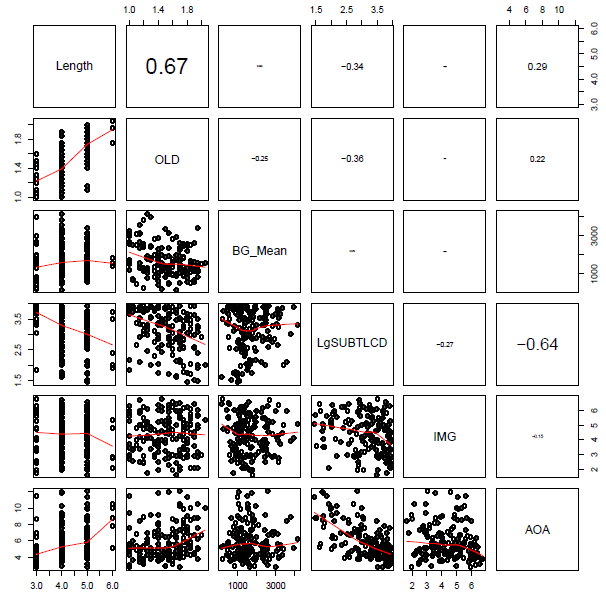
# draw a pairs scatterplot matrix

pdf("ML-nomissing-full-pairs-items-splom-110513.pdf", width = 8, height = 8)

pairs(nomissing.full.pairs.items, lower.panel=panel.smooth, upper.panel=panel.cor)

dev.off()

# draw a pairs scatterplot matrix

pdf("ML-nomissing-full-pairs-subjects-splom-110513.pdf", width = 8, height = 8)

pairs(nomissing.full.pairs.subjects, lower.panel=panel.smooth, upper.panel=panel.cor)

dev.off()

# assess collinearity using the condition number, kappa, metric

collin.fnc(nomissing.full.pairs.items)$cnumber
collin.fnc(nomissing.full.pairs.subjects)$cnumber

# > collin.fnc(nomissing.full.pairs.items)$cnumber
# [1] 46.0404
# > collin.fnc(nomissing.full.pairs.subjects)$cnumber
# [1] 36.69636

You will see when you run this code that the set of subject attribute predictors (see below) …

… and the set of item attribute predictors (see below) …

… include some quite strongly overlapping variables, distinguished by high correlation coefficients.

I was advised, when I started doing regression analyses, that a rule-of-thumb one can happily use when examining bivariate i.e. pairwise correlations between predictor variables is that there is no multicollinearity to worry about if there are no coefficients greater than $r = .8$ however, I can think of no statistical reason for this number, while Baayen (2008) recommends using the condition number, kappa, as a diagnostic measure, based on Belsley et al.’s (1980) arguments that pairwise correlations do not reveal the real, underlying, structure of latent factors (i.e. principal components of which collinear variables are transformations or expressions).

If we calculate the condition number for, separately, the subject predictors and the item predictors, we get values of 30+ in each case. Baayen (2008) comments that (if memory serves) a condition number higher than 12 indicates a dangerous level of multicollinearity. However, Cohen et al. (2003) comment that while 12 or so might be a risky kappa there are no strong statistical reasons for setting the thresholds for a ‘good’ or a ‘bad’ condition number; one cannot apply the test thoughtlessly. That said, 30+ does not look good.

The condition number is based around Principal Components Analysis (PCA) and I think it is worth considering the outcome of such an analysis over predictor variables when examining the multicollinearity of those variables. PCA will often show that set of several item attribute predictors will often relate quite strongly to a set of maybe four orthogonal components: something to do with frequency/experience; something relating to age or meaning; something relating to word length and orthographic similarity; and maybe some thing relating to sublexical unit frequency. However, as noted previously, Cohen et al. (2003) provide good arguments for being cautious about performing a principal components regression in response to a state of high collinearity among your predictors, including problems relating to the interpretability of findings.

Center variables on their means

One perhaps partial means to alleviate the collinearity indicated may be to center predictor variables on their means.

(Should you center variables on their means before or after you remove errors, i.e. means calculated for the full or the no-errors dataframe? Should you center both predictors and the outcome variables? I will need to come back to those questions.)

Centering variables is helpful, also, for the interpretation of effects where 0 on the raw variables is not meaningful e.g. noone has an age of 0 years, no word has a length of 0 letters. With centered variables, if there is an effect then one can say that for unit increase in the predictor variable (where 0 for the variable is now equal to the mean for the sample, because of centering), there is a change in the outcome, on average, equal to the coefficient estimated for the effect.

Centering variables is helpful, especially, when we are dealing with interactions. Cohen et al. (2003) note that the collinearity between predictors and interaction terms is reduced (this is reduction of nonessential collinearity, due to scaling) if predictors are centered. Note that interactions are represented by the multiplicative product of their component variables. You will often see an interaction represented as “age x word length effects”, the “x” reflects the fact that for the interaction of age by length effects the interaction term is entered in the analysis as the product of the age and length variables. In addition, centering again helps with the interpretation of effects because if an interaction is significant then one must interpret the effect of one variable in the interaction while taking into account the other variable (or variables) involved in the interaction (Cohen et al., 2003; see, also, Gelman & Hill, 2007). As that is the case, if we center our variables and the interaction as well as the main effects are significant, say, in our example, the age, length and age x length effects, then we might look at the age effect and interpret it by reporting that for unit change in age the effect is equal to the coefficient while the effect of length is held constant (i.e. at 0, its mean).

As you would expect, you can center variables in R very easily, we will use one method, which is to employ the scale() function, specifying that we want variables to be centered on their means, and that we want the results of that operation to be added to the dataframe as centered variables. Note that by centering on their means, I mean we take the mean for a variable and subtract it from each value observed for that variable. We could center variables by standardizing them, where we both subtract the mean and divide the variable by its standard deviation (see Gelman & Hill’s 2007, recommendations) but we will look at that another time.

So, I center variables on their means, creating new predictor variables that get added to the dataframe with the following code:


# we might center the variables - looking ahead to the use of interaction terms - as the centering will
# both reduce nonessential collinearity due to scaling (Cohen et al., 2003) and help in the interpretation
# of effects (Cohen et al., 2003; Gelman & Hill, 2007 p .55) ie if an interaction is sig one term will be
# interpreted in terms of the difference due to unit change in the corresponding variable while the other is 0

nomissing.full$cLength <- scale(nomissing.full$Length, center = TRUE, scale = FALSE)
nomissing.full$cBG_Mean <- scale(nomissing.full$BG_Mean, center = TRUE, scale = FALSE)
nomissing.full$cOLD <- scale(nomissing.full$OLD, center = TRUE, scale = FALSE)
nomissing.full$cIMG <- scale(nomissing.full$brookesIMG, center = TRUE, scale = FALSE)
nomissing.full$cAOA <- scale(nomissing.full$AoA_Kup_lem, center = TRUE, scale = FALSE)
nomissing.full$cLgSUBTLCD <- scale(nomissing.full$LgSUBTLCD, center = TRUE, scale = FALSE)

nomissing.full$cAge <- scale(nomissing.full$Age, center = TRUE, scale = FALSE)
nomissing.full$cTOWREW <- scale(nomissing.full$TOWRE_wordacc, center = TRUE, scale = FALSE)
nomissing.full$cTOWRENW <- scale(nomissing.full$TOWRE_nonwordacc, center = TRUE, scale = FALSE)
nomissing.full$cART <- scale(nomissing.full$ART_HRminusFR, center = TRUE, scale = FALSE)

# subset the predictors again by items and person level attributes to make the plotting more sensible

nomissing.full.c.items <- subset(nomissing.full, select = c(

 "cLength", "cOLD", "cBG_Mean", "cLgSUBTLCD", "cIMG", "cAOA"

))

nomissing.full.c.subjects <- subset(nomissing.full, select = c(

 "cAge", "cTOWREW", "cTOWRENW", "cART"

))

# assess collinearity using the condition number, kappa, metric

collin.fnc(nomissing.full.c.items)$cnumber
collin.fnc(nomissing.full.c.subjects)$cnumber

# > collin.fnc(nomissing.full.c.items)$cnumber
# [1] 3.180112
# > collin.fnc(nomissing.full.c.subjects)$cnumber
# [1] 2.933563

Notice:

— I check the condition numbers for the predictors after centering and it appears that they are significantly reduced.

— I am not sure that that reduction can possibly be the end of the collinearity issue, but I shall take that result and run with it, for now.

— I also think that it would be appropriate to examine collinearity with both the centered variables and the interactions involving those predictors but that, too, can be left for another time.

Run the models

What I will do next is perform three sets of mixed-effects model analyses. I will talk about the first set in this post.

In this first set, I shall compare models varying in the predictor variables included in the model specification. We shall say that models with more predictors are more complex than models with fewer predictors (a subset of the predictors specified for the more complex models).

I shall then compare models of differing in complexity to see if increased complexity is justified by improved fit to data.

This is in response to: 1. reading Baayen (2008) and Pinheiro & Bates (2000) 2. recommendations by a reviewer; though I note that the reviewer recommendations are, in their application, qualified in my mind by some cautionary comments made by Pinheiro & Bates (2000), and confess that any problems of application or understanding are surely expressions of my misunderstanding.

What I am concerned about is the level of complexity that can be justified in the ultimate model by the contribution to improved fit by the model of the observed data. Of course, I have collected a set of predictors guided by theory, custom and practice in my field. But, as you have seen, I might choose to draw on a large set of potential predictors. I know that one cannot – to take one option used widely by psycholinguistics researchers – simply inspect a correlation table, comparing predictors with the outcome variable, and exclude those predictors that do not correlate with the outcome. Harrell (2001) comments that that approach has a biasing effect on the likelihood of detecting an effect that is really there (consuming, ‘ghost degrees of freedom’, or something like that). So what should we do or how should we satisfy ourselves that we should or should not include one or more predictor variables in our models?

You could start complex and step backwards to the simplest model that appears justified by model fit to observed data. I will return to that option another time.

In this post, I will start with the simplest model and build complexity up. Simpler models can be said to be nested in more complex models, e.g. a simple model including just main effects vs. a more complex model also including interactions. I will add complexity by adding sets of predictors, and I will compare each proximate pair of simple model and more complex model using the Likelihood Ratio Test (Pinheiro & Bates, 2000; see, especially, chapter 2, pp. 75-).

We can compare models with the same random effects (e.g. of subjects or items) but varying in complexity with respect to the fixed effects, i.e. replicable or manipulated variables like item length or participant age, and, separately, models with the same fixed effects but varying random effects.

Note that in comparing models varying in random effects, one estimates those effects using restricted maximum likelihood: you will see the argument REML = TRUE in the lmer() function call, that is what REML means. Note that in comparing models varying in fixed effects one must estimate those effects using maximum likelihood: you will see the argument REML = FALSE in the lmer() function call, that is what FALSE means. See comments in Baayen (2008) and Pinheiro & Bates (2000); I will come back to those important terms to focus on understanding, another time, focusing in this post on just writing the code for running the models.

We can compare the more and less complex models using the Likelihood Ration Test (LRT) which is executed with the anova([simple model], [more complex model]) function call. A $\chi^2$ statistic is computed, and evaluated against the $\chi^2$ distribution to estimate the probability of an increase in model likelihood as large or larger as that observed when comparing the more or less complex model, given the null hypothesis of no gain in likelihood.

Note that I log transform the RTs but one might also consider examining the reciprocal RT.


# we can move to some multilevel modelling ###############################################################

# we might start by examining the effects of predictors in a series of additions of sets of predictors
# we can hold the random effects, of subjects and items, constant, while varying the fixed effects
# we can compare the relative fit of models to data using the anova() likelihood ratio test
# in this series of models, we will use ML fitting

full.lmer0 <- lmer(log(RT) ~

# Trial.order +
#
# cAge + cTOWREW + cTOWRENW + cART +
#
# cLength + cOLD + cBG_Mean + cLgSUBTLCD + cAOA + cIMG +

 (1|subjectID) + (1|item_name),

 data = nomissing.full, REML = FALSE)

print(full.lmer0,corr=F)

#

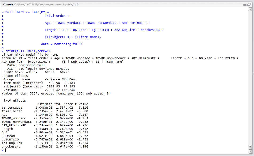
full.lmer1 <- lmer(log(RT) ~

 Trial.order +

 # cAge + cTOWREW + cTOWRENW + cART +
 #
 # cLength + cOLD + cBG_Mean + cLgSUBTLCD + cAOA + cIMG +

 (1|subjectID) + (1|item_name),

 data = nomissing.full, REML = FALSE)

print(full.lmer1,corr=F)

#

full.lmer2 <- lmer(log(RT) ~

 Trial.order +

 cAge + cTOWREW + cTOWRENW + cART +

 # cLength + cOLD + cBG_Mean + cLgSUBTLCD + cAOA + cIMG +

 (1|subjectID) + (1|item_name),

 data = nomissing.full, REML = FALSE)

print(full.lmer2,corr=F)

#

full.lmer3 <- lmer(log(RT) ~

 Trial.order +

 cAge + cTOWREW + cTOWRENW + cART +

 cLength + cOLD + cBG_Mean + cLgSUBTLCD + cAOA + cIMG +

 (1|subjectID) + (1|item_name),

 data = nomissing.full, REML = FALSE)

print(full.lmer3,corr=F)

#

full.lmer4 <- lmer(log(RT) ~

 Trial.order +

 (cAge + cTOWREW + cTOWRENW + cART)*

 (cLength + cOLD + cBG_Mean + cLgSUBTLCD + cAOA + cIMG) +

 (1|subjectID) + (1|item_name),

 data = nomissing.full, REML = FALSE)

print(full.lmer4,corr=F)

# compare models of varying complexity

anova(full.lmer0, full.lmer1)
anova(full.lmer1, full.lmer2)
anova(full.lmer2, full.lmer3)
anova(full.lmer3, full.lmer4)

This code will first print out the summaries of each model, along the lines you have already seen. It will then give you this:


# > # compare models of varying complexity
# >
# > anova(full.lmer0, full.lmer1)
# Data: nomissing.full
# Models:
# full.lmer0: log(RT) ~ (1 | subjectID) + (1 | item_name)
# full.lmer1: log(RT) ~ Trial.order + (1 | subjectID) + (1 | item_name)
# Df AIC BIC logLik Chisq Chi Df Pr(>Chisq)
# full.lmer0 4 -977.58 -951.31 492.79
# full.lmer1 5 -975.83 -943.00 492.92 0.2545 1 0.6139
# > anova(full.lmer1, full.lmer2)
# Data: nomissing.full
# Models:
# full.lmer1: log(RT) ~ Trial.order + (1 | subjectID) + (1 | item_name)
# full.lmer2: log(RT) ~ Trial.order + cAge + cTOWREW + cTOWRENW + cART + (1 |
# full.lmer2: subjectID) + (1 | item_name)
# Df AIC BIC logLik Chisq Chi Df Pr(>Chisq)
# full.lmer1 5 -975.83 -943.00 492.92
# full.lmer2 9 -977.09 -917.98 497.54 9.2541 4 0.05505 .
# ---
# Signif. codes: 0 ‘***’ 0.001 ‘**’ 0.01 ‘*’ 0.05 ‘.’ 0.1 ‘ ’ 1
# > anova(full.lmer2, full.lmer3)
# Data: nomissing.full
# Models:
# full.lmer2: log(RT) ~ Trial.order + cAge + cTOWREW + cTOWRENW + cART + (1 |
# full.lmer2: subjectID) + (1 | item_name)
# full.lmer3: log(RT) ~ Trial.order + cAge + cTOWREW + cTOWRENW + cART + cLength +
# full.lmer3: cOLD + cBG_Mean + cLgSUBTLCD + cAOA + cIMG + (1 | subjectID) +
# full.lmer3: (1 | item_name)
# Df AIC BIC logLik Chisq Chi Df Pr(>Chisq)
# full.lmer2 9 -977.09 -917.98 497.54
# full.lmer3 15 -1115.42 -1016.91 572.71 150.34 6 < 2.2e-16 ***
# ---
# Signif. codes: 0 ‘***’ 0.001 ‘**’ 0.01 ‘*’ 0.05 ‘.’ 0.1 ‘ ’ 1
# > anova(full.lmer3, full.lmer4)
# Data: nomissing.full
# Models:
# full.lmer3: log(RT) ~ Trial.order + cAge + cTOWREW + cTOWRENW + cART + cLength +
# full.lmer3: cOLD + cBG_Mean + cLgSUBTLCD + cAOA + cIMG + (1 | subjectID) +
# full.lmer3: (1 | item_name)
# full.lmer4: log(RT) ~ Trial.order + (cAge + cTOWREW + cTOWRENW + cART) *
# full.lmer4: (cLength + cOLD + cBG_Mean + cLgSUBTLCD + cAOA + cIMG) +
# full.lmer4: (1 | subjectID) + (1 | item_name)
# Df AIC BIC logLik Chisq Chi Df Pr(>Chisq)
# full.lmer3 15 -1115.4 -1016.91 572.71
# full.lmer4 39 -1125.7 -869.56 601.84 58.262 24 0.0001119 ***
# ---
# Signif. codes: 0 ‘***’ 0.001 ‘**’ 0.01 ‘*’ 0.05 ‘.’ 0.1 ‘ ’ 1

# it looks like the full model, including interactions but not the trialorder variable, is justified

Notice:

— It is not very pretty but it does tell you what predictors are included in each model you are comparing, for each pair of models being compared, the outcome of the ratio test, giving the numbers I usually report: the $\chi^2, df$ and the $p-value$ .

— I am looking at this output to see if, for each pair of models, the more complex model fits the data significantly better (if p =< 0.05).

–I add predictors in blocks and assess the improvement of fit associated with the whole block.

I have made a lot of promises to explain things more another time. So I will add one more. Pinheiro & Bates (2000; p. 88) argue that Likelihood Ratio Test comparisons of models varying in fixed effects tend to be anticonservative i.e. will see you observe significant differences in model fit more often than you should. I think they are talking, especially, about situations in which the number of model parameter differences (differences between the complex model and the nested simpler model) is large relative to the number of observations. This is not really a worry for this dataset, but I will come back to the substance of this view, and alternatives to the approach taken here.

Get the p-values

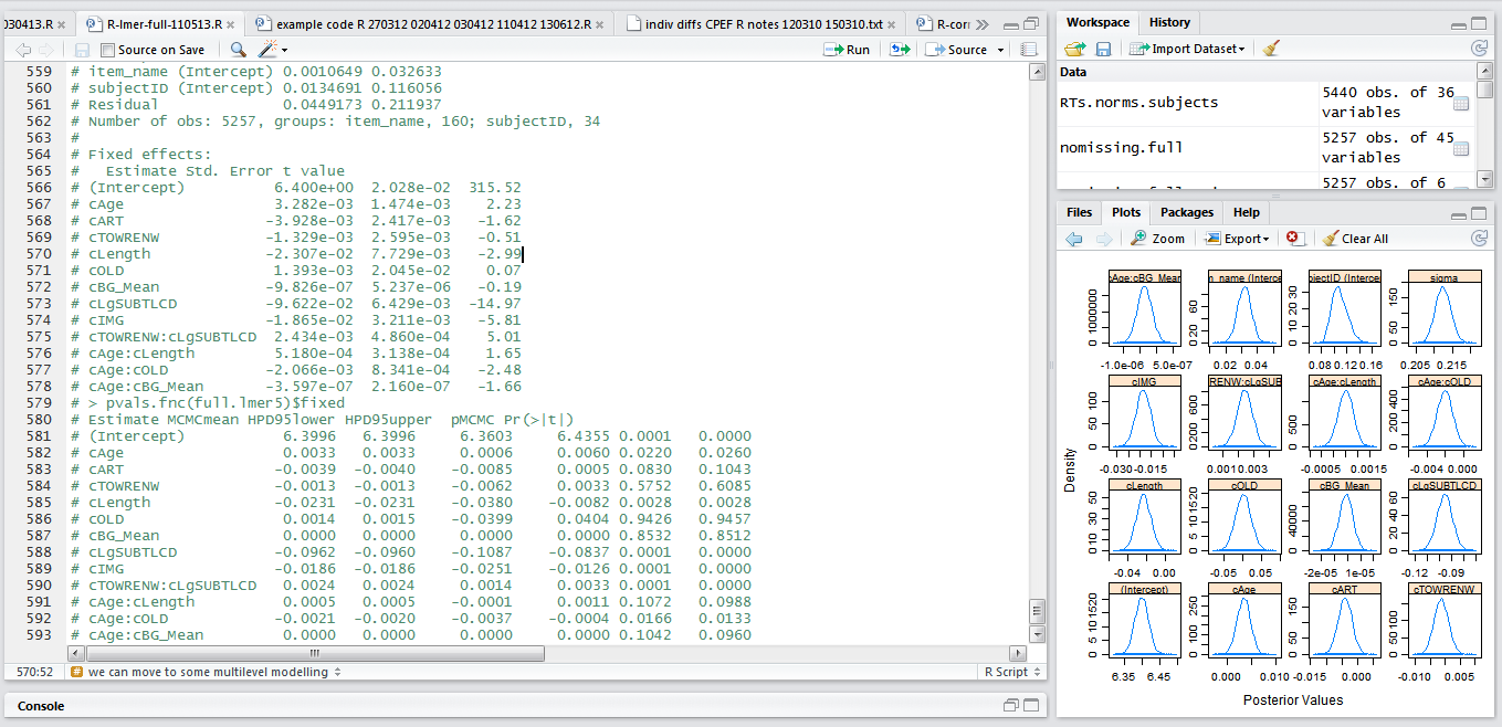
Finally, we request the generation of p-values for the effects we have entered in the model with the most justifiable complexity.


# get p-values

full.lmer4 <- lmer(log(RT) ~

 Trial.order +

 (cAge + cTOWREW + cTOWRENW + cART)*

 (cLength + cOLD + cBG_Mean + cLgSUBTLCD + cAOA + cIMG) +

 (1|subjectID) + (1|item_name),

 data = nomissing.full, REML = FALSE)

print(full.lmer4,corr=F)
pvals.fnc(full.lmer4)$fixed

and the combination of the last commands, to print a summary of the model, and to calculate p-values, will tell you that:-

— We have significant effects due to:

cAge + cART + cTOWRENW +

cLength + cOLD + cBG_Mean + cLgSUBTLCD + cIMG +

cTOWRENW:cLgSUBTLCD + cAge:cLength + cAge:cOLD + cAge:cBG_Mean

I am writing the interactions not as var1*var2 but as var1:var2 – the second form of expressing an interaction restricts the analysis to considering just that product term whereas the first requires the analysis to consider the products and all its components. We must, if include an interaction in our model also include all its main effects components – try not doing this, you should get an error – however, I have found that if you were to include e.g. age*length and also age*OLD there are problems while the more restrictive age:length and age:OLD seems to deal with that problem. I have a feeling Baayen (2008) explains this better but I do not have a copy to hand and therefore cannot relay his explanation here.

— The initial summary of the model shows fixed and random effects estimates but does not give you p-values. Baayen et al. (2008) explain that if we were doing ordinary least squares regression, the method for calculating p-values has been well worked out, assuming just the fixed effects plus a single parameter corresponding to random (normally distributed) error, with a calculation of model degrees of freedom corresponding to estimated effects and residual degrees of freedom corresponding to the number of observations less the number of effects. It is hard to calculate degrees of freedom for mixed-effects models: should we count the number of subjects, or of items, or, somehow, both?

— Baayen et al. (2008) argue that what we want is to understand the imprecision of our estimate of the random errors when looking at our fixed effects. This is what we can achieve with Markov chain Monte Carlo simulations, the source of the p-values we report.

— The t- and MCMC-derived p-values will tend to coincide for most analyses.

— We get significant effects that appear to make sense: effects of age, reading experience, length (though longer words elicit shorter RTs), frequency, AoA (near significant), imageability, and interactions between age and length, age and Orthographic Levenshtein Distance (OLD), age and mean bigram frequency, nonword reading skill and frequency.

What next?

What I would seek to do in the next series of analyses is determine if the effects that are significant appear to be significant due:

1. to the presence of other, nonsignificant effects — making the check by removing the nonsignificant effects then rerunning the model;

2. to the presence of outlier observations — making the check by removing observations associated with large model residuals then rerunning the model.

What have we learnt?

(The code I have used in running the analysis described in this post can be found here.)

Firstly, I am going to have to do a lot more explaining, for my own sake, and have promised to do so for a wide range of ideas, including those concerning the methods of model fitting, and, especially, the discussion around how one determines the appropriate set of fixed effects.

Secondly, that the model code is both simple and – on its face – reasonably intuitive.

Key vocabulary (mostly, a list of things to be explained)

fixed effects

random effects

random intercepts

random slopes

interactions

multiplicative products

centering

maximum likelihood

restricted maximum likelihood

Markov chain Monte Carlo

Likelihood Ratio Test

lmer()

anova()

pvals.fnc()

Reading

Baayen, R. H. (2008). Analyzing linguistic data. Cambridge University Press.
Bates, D. M. (2005). Fitting linear mixed models in R. R News, 5, 27-30.
Belsley, D. A., Kuh, E., & Welsch, R. E. (1980). Regression diagnostics: Identifying influential data and sources of collinearity. New York: Wiley.
Cohen, J., Cohen, P., West, S. G., & Aiken, L. S. (2003). Applied multiple regression/correlation analysis for the behavioural sciences (3rd. edition). Mahwah, NJ: Lawrence Erlbaum Associates.
Gelman, A., & Hill, J. (2007). Data analysis using regression and multilevel/hierarchical models. New York,NY: Cambridge University Press.
Pinheiro, J. C., & Bates, D. M. (2000). Mixed-effects models in S and S-plus (Statistics and Computing). New York: Springer.

Posted in 16. Modelling - mixed-effects | Tagged AIC, anova(), BIC, chi-sq, fixed effects, lmer(), MCMC, random effects | Leave a comment

Modelling – example mixed-effects analysis

Posted on May 10, 2013 by robayedavies

In the last post, I showed how to collate the various data bases we constructed or collated from the data collection achieved in a study of lexical decision. We ended the post by producing a .csv file of the output of our various merger operations, which can be downloaded here.

This file holds data on:

1. participant attributes;

2. word attributes;

3. participant responses to words in the lexical decision task.

In this post, I want to take a quick look at how you would actually run a mixed-effects model, using the lmer() function furnished by the lme4 package, written by Doug Bates (Bates, 2010 – appears to a preprint of his presumed new book, see also Pinheiro & Bates, 2000). A useful how-to guide, one I followed when I first started doing this kind of modelling, is in Baayen (2008). An excellent, and very highly cited, introduction to mixed-effects modelling for psycholinguistics, is found in Baayen, Davidson & Bates (2008).

Creative commons – flickr – LIGC-NLW: village of Oystermouth from the castle window (Mary Dillwyn, 1854)

First, then, we enter the following lines of code to load the libraries we are likely to need, to set the working directory to the folder where we have copied the full database, and to read that database as a dataframe in the session’s workspace:


library(languageR)
library(lme4)
library(ggplot2)
library(grid)
library(rms)
library(plyr)
library(reshape2)
library(psych)
library(gridExtra)

# set the working directory

setwd("C:/Users/p0075152/Dropbox/resources R public")

# read in the full database

item.words.norms <- read.csv("RTs.norms.subjects 090513.csv", header=T, na.strings = "-999")

We should then inspect what we get:


# inspect the dataframe

head(RTs.norms.subjects, n = 2)
summary(RTs.norms.subjects)
describe(RTs.norms.subjects)
str(RTs.norms.subjects)
length(RTs.norms.subjects)
length(RTs.norms.subjects$item_name)
levels(RTs.norms.subjects$item_name)

If we consider the output from the summary() function call, we can see mostly what we expect and one thing we need to deal with before we do any modelling:

Notice:

— The minimum value for the RT variable is -2000. Negative RTs arise because DMDX will record a correct response as a positive and an incorrect response as a negative number, and we did not deal with that fact through the whole data collation process.

In fact, having incorrect responses associated with negative RTs is useful because we can subset the dataframe, setting a condition on rows, to remove all observations pertaining to errors.


nomissing.full <- RTs.norms.subjects[RTs.norms.subjects$RT > 0,]

summary(nomissing.full)

You will see, if you run those lines, that the summary of the new no missing i.e. no errors dataframe has 5257 rows, the ones we lost are the errors, as we can see that the minimum RT is now 262.2 (might be worth considering if that RT is too small, a recording error, another time).

We can then move on to run the mixed-effects model:


full.lmer1 <- lmer(RT ~
 Trial.order +

 Age + TOWRE_wordacc + TOWRE_nonwordacc + ART_HRminusFR +

 Length + OLD + BG_Mean + LgSUBTLCD + AoA_Kup_lem + brookesIMG +

 (1|subjectID) + (1|item_name),

 data = nomissing.full)

print(full.lmer1,corr=F)

Notice:
— We are running the model using the lmer() function.

— We specify that the dataframe in play is the nomissing.full one we just created.

— We created a model, the object assigned to a name full.lmer1, with the lmer() function call.

— We later output a summary of that model using the print() function call; no output would be shown otherwise.

— The model has the following components:

1. RT — the outcome or dependent variable

2. ~ — predicted by

3. A set of predictors including:

Trial.order +

Age + TOWRE_wordacc + TOWRE_nonwordacc + ART_HRminusFR +

Length + OLD + BG_Mean + LgSUBTLCD + AoA_Kup_lem + brookesIMG +

— the fixed effects.

4. A set of predictors also including:

(1|subjectID) + (1|item_name)

— the random effects, here, random effects due to participant and item effects on intercepts.

The output summary of this model is shown in the R-studio console window as:

Notice:

— We do not get p-values.

— We are shown the estimated spread of random effects.

— We are shown the fixed effects in a format equivalent to the coefficients summary table for a regression analysis.

— Knowing that if $t >= 2$ then we can see that there are a number of significant effects:

1. Age — older readers had slower RTs;

2. ART score — more experienced readers were faster;

3. Length — longer words elicited shorter RTs;

4. Frequency – LgSUBTLCD — more frequent words elicited shorter RTs;

5. Imageability – IMG – more imageable words elicited shorter RTs.

Aside from the length effect which contrasts with some previous reports (Weeks, 1997) but not others (New et al., 2007), these effects are consistent with numerous previous observations in the literature.

We could take these results to a report, if we wanted.

Obviously, however, what we will do in later posts will be to consider how we can examine and display the utility and the validity of this model, and models like it.

What have we learnt?

(The code used to run the model can be found here.)
Well, not much, just how to run a lmer() mixed-effects model. The real work is just starting.

Key vocabulary

lmer()

Reading

Baayen, R. H. (2008). Analyzing linguistic data. Cambridge University Press.
Baayen, R. H., Davidson, D. J., & Bates, D. M. (2008). Mixed-effects modeling with crossed random effects for subjects and items. Journal of Memory and Language, 59, 390-412.
Balota, D., Cortese, M. J., Sergent-Marshall, S. D., Spieler, D., & Yap, M. (2004). Visual word recognition of single-syllable words. Journal of Experimental Psychology: General, 133, 283-316.
Bates, D. M. (2005). Fitting linear mixed models in R. R News, 5, 27-30.
New, B., Ferrand, L., Pallier, C., & Brysbaert, M. (2007). Re-examining the word length effect in visual word recognition: New evidence from the English lexicon project. Psychonomic Bulletin and Review, in press
Pinheiro, J. C., & Bates, D. M. (2000). Mixed-effects models in S and S-plus (Statistics and Computing). New York: Springer.
Weekes, B. S. (1997). Differential effects of number of letters on word and nonword naming latency. The Quarterly Journal Of Experimental Psychology, 510A 439-456.

Posted in 16. Modelling - mixed-effects | Tagged lmer() | Leave a comment

Modelling – look ahead to mixed-effects modelling

Posted on May 10, 2013 by robayedavies

So far, we have been looking at the participant attributes or the item attributes for our lexical decision study. It is time to move on to consider a mixed-effects analysis examining whether or how lexical decision responses were influenced by:

1. the participant attributes;

2. the item attributes;

3. interactions between participant and item attributes.

In this post, we will consider how we put together all the bits of data we collected in the course of the study. In the next post, we will do a bit of modelling to give the mixed-effects modelling syntax a run out, we will then work our way carefully through the process to make sure everything is understood, and that the model we end up with is the ‘best’ (and we shall consider how to evaluate that).

Creative commons – flickr – LIGC-NLW: Harry and Amy Dillwyn (taken by Mary Dillwyn, 1853)

To examine the behaviour in the lexical decision study, we will need to bring in the behavioural data that we collected.

It is worth reminding ourselves of how we got these data.

Lexical decision study summary

We tested 39 adults, males and females, most either in their 20s or in middle age.

Every adult was tested on word and nonword reading skills (TOWRE, Torgesen et al., 1999) and print exposure (ART, Masterson & Hayes, 2007). We collated the subject scores database and it can be downloaded here.

Critically, every adult also was tested in a computer based lexical decision task (run using DMDX, Forster & Forster, 2003) in which they saw 320 letter strings on a screen, one at a time, and were asked to indicate by a button press (using a gamepad) whether they thought each item was a word they knew or a nonword they did not. In addition to the 320 critical trials, participants were also given 20 practice trials which we shall ignore in the analysis.

The words and nonwords were selected to be matched on length (measured in letters), orthographic neighbourhood size (often called N, Coltheart et al., 1977) and bigram frequency (mean, sum and frequency specific numbers). This matching was designed to force participants to access their mental lexicon to perform the task, instead of making responses based on ‘low-level’ perceptual information like item length. We collated data on item (word and nonword attributes) and they can be downloaded here, see relevant previous posts here and here.

However, what we really cared about, in designing the experiment, was whether the time that participants took to respond to stimuli (reaction time, RT, or response latency) – the interval from stimulus onset to response onset – varied in relation to: participant attributes like reading skill; item attributes like length; and the interactions between those two sets of predictors. In addition to the length etc. of the items, we also cared if lexical access was influenced by word attributes. Focusing on just words, we wanted to know if RTs were affected by word frequency, age of acquisition (AoA), and imageability. We collated information about such attributes and combined them with data on item attributes like length to a single database that can be downloaded here, see relevant post here.

All these data about item attributes were drawn either from the English Lexicon Project (Balota et al., 2007) or from datasets very helpfully provided by other psycholinguists (Cortese & Fuggett, 2004; Cortese & Khanna, 200; Kuperman et al., in press) see notes here and here.

When we ran the lexical decision study, DMDX produced an .azk output file holding keypress RTs along with information about trial order (when did a word appear in a block of stimulus trials) and participant identity code (subjectID).

Getting data recorded in an experiment into a usable state can be a quite exasperating process. Things that one encounters include: inconsistent subjectID naming between behavioural and participant attribute data collection; item or trial coding errors; mismatches because one used the word false in excel. For some reason, the process of data collation is often called data munging.

The behavioural data file is in ‘long format’: all participants tested are shown, one participant on top of the other, in a long column where each row corresponds to a single trial observation, i.e. each row corresponds to a response made by a participant to a word. It can be downloaded here.

If you open it in excel, it looks like this:

Notice:

— If you were to open the file in excel, you would see that there are 13941 rows, including the column headers or variable names.

— 13940 data rows = 340*41

– Recall I said there were 320 critical trials and 39 participants. On the latter score, I misspoke: we lost two because of inconsistent subjectID entry. If you don’t know who they are (or, at least, if you cannot map subjectIDs in a participant attributes to subjectIDs in a behavioural database), you cannot analyze them.

Load the data into the workspace

I am going to assume you have successfully downloaded the datafiles and have them in a folder that you are able to use as your working directory.

You can run the following code to set the working directory to the folder where the datafiles are and then load the files into the R session workspace as dataframes.


# set the working directory

setwd("C:/Users/p0075152/Dropbox/resources R public")

# # read in the item norms data
#
# item.norms <- read.csv(file="item norms 270312 050513.csv", head=TRUE,sep=",", na.strings = "-999")
# word.norms <- read.csv(file="word norms 140812.csv", head=TRUE,sep=",", na.strings = "-999")

item.coding <- read.csv(file="item coding info 270312.csv", head=TRUE,sep=",", na.strings = "-999")

# read in the merged new dataframe

item.words.norms <- read.csv(file="item.words.norms 050513.csv", head=TRUE,sep=",", na.strings = "NA")

# read in the subjects scores data file

subjects <- read.csv("ML scores 080612 220413.csv", header=T, na.strings = "-999")

# read in the behavioural data file

behaviour <- read.csv("ML data 080612.csv", header=T, na.strings = "-999")

Notice:

— I commented out the read.csv() function calls for item.norms and word.norms. We will not need that stuff for this post.

— We do now need the item.coding dataframe, however, for reasons I will explain next.

Put the databases together

We next need to put the dataframes together through the use of the merge() function.

What this means is that we will end up with a dataframe that:

1. has as many rows (some thousands) as valid observations

2. each observation will be associated with data about the subject and about the word.

Notice:

— The merge() function (see the help page) allows you to put two dataframes together. I believe other functions allow merger of multiple dataframes.

— By default, the dataframes are merged on the columns with names they both have, so here we plan to merge: the normative item.words.norms dataframe with the item.coding dataframe by the common variable item_name; we then merge that norms.coding dataframe with the behaviour dataframe by the common variable item_number; we then merge that RTs.norms dataframe with the subject scores dataframe by the common variable subjectID.

— You see why we needed the coding data: the behavioural database lists RT observations by (DMDX trial item) number; the normative database lists item attribute observations by item name (e.g. a word name like “axe”); I cannot put the normative and the behavioural databases without a common variable, that common variable has to be item_name so I created the coding database, deriving the information from the DMDX script, to hold both the item_name and item_number columns. Creating the coding database was not too costly but the fact that I needed to do so illustrates the benefits of thinking ahead, if I had thought ahead, I would have had both item_name and item_number columns in the normative database when I built it.

— As noted previously, if the dataframes being merged do not have observations that cannot be mapped together because there is a mismatch on the row index e.g. item name or whatever other common variable is being used they get ‘lost’ in the process of merging. This is nicely illustrated by what happens when you merge the behaviour dataframe – which holds observations on both responses to words and to nonwords – with the item.words.norms dataframe, which holds just data about the attributes of words. As there are no nonword items in the latter, when you merge item.words.norms and behaviour, creating a new joint dataframe, the latter has nothing about nonwords. This suits my purposes, because I wish to ignore nonwords (and practice items, for that matter, also absent from the norms database) but you should pay careful attention to what should happen and what does happen when you merge dataframes.

— I also check my expectations about the results of operations like merge() against the results of those operations. I almost never get a match first time between expectations and results. Here, it is no different, as I will explain.

Let’s run the code to merge our constituent databases.


# to put files together ie to merge files we use the merge() function
# we want to put the data files together so that we can analyze RTs by subject characteristics or item norms or conditions (coding)

# so that we can associate item normative with coding data, we need to merge files by a common index, item_name

norms.coding <- merge(item.words.norms, item.coding, by="item_name")

# inspect the result

head(norms.coding, n = 2)

# note the common index item_name does not get repeated but R will recognize the duplication of item_type and assign .x or .y
# to distinguish the two duplicates.

# delete the redundant column

norms.coding <- norms.coding[, -2] # using data file indexing, [,] - to remove, remove 2 the second column

head(norms.coding,n=2)

# rename the .y column to keep it tidy

norms.coding <- rename(norms.coding, c(item_type.y = "item_type"))

# inspect the results:

head(norms.coding,n=2)

summary(norms.coding)

# put the data files together with data on subjects and on behaviour:

# first, rename "Item" variable in lexical.RTs as "item_number" to allow merge

behaviour <- rename(behaviour, c(Item = "item_number"))

# run merge to merge behaviour and norms

RTs.norms <- merge(norms.coding, behaviour, by="item_number")

# run merge to merge RTs.norms and subject scores

RTs.norms.subjects <- merge(RTs.norms, subjects, by="subjectID")

Notice:

— In merging the normative and coding dataframes, I had to deal with the fact that both held two common columns, the one I used for merging, item_name, and another, item_type. The former is used for merging and goes into the dataframe that is the product of the merger as a single column. The item_type column was not used for merging and consequently is duplicated: R deals with duplicates by renaming them to keep them distinct, here adding .x or .y. This is a bit of a pain so I dealt with the duplication by deleting one copy and renaming the other.

If we inspect the results of the merger:


# inspect the results:

head(RTs.norms.subjects,n=2)
summary(RTs.norms.subjects)
length(RTs.norms.subjects$RT)

We see:

Notice:

— We have just observations of words: see the item_type summary.

— Participants, at least the first few, are listed under subjectID with 160 observations each, as they should be. Variables appear to be correctly listed by data type, numeric, factor etc.

— I note that there are some missing values, NAs, among the IMG and AOA observations.

— I also note that the Subject variable indicates at least one participant, A18, has 320 not 160 observations.

Checking: Does the merger output dataframe match my expectations?

As noted in the foregoing study summary, we have participant attribute data on 39 participants and, presumably, lexical decision behavioural data on those same participants. I would expect the final merger output dataframe, therefore, to have: 39*160 = 6240 rows.

It does not.

We need to work out what the true state of each component dataframe is to make sense of what we get as the output of the merge() calls.

The first thing I am going to do is to check if the merger between subjects and behaviour dataframes lost a few observations because there was a mismatch on subjectID for one or more participants. The way you can do this (there are smarter ways) is ask R what the levels of the subjectID factor are for each dataframe then check the matching by eye.


# how many rows should we have?

levels(subjects$subjectID)
levels(behaviour$subjectID)
levels(RTs.norms.subjects$subjectID)

Which shows you this:

I can tell that there are some subjectIDs in the subjects dataframe that are not in the behaviour dataframe, and vice versa. Well, I told you that there were problems in the consistency of subjectID naming. The output dataframe RTs.norms.subjects will only have observations for those rows indexed with a subjectID in common between both behaviour and subjects dataframes. (I think the smarter way to do the check would be to do a logic test, using ifelse(), with a dataframe output telling you where subjectID is or is not matched.)

Notice:

— The behaviour dataframe includes 41 not 39 participants’ data, including one with a blank “” subjectID.

— The levels listed for subjectID for the output dataframe RTs.norms.subjects actually gives you all levels listed for both factors, irrespective of whether there are other data associated with each level. This is an artifact of the way in which R (otherwise efficiently) stores factors as indices, with instances.

— We need, therefore, to count how many observations we have for each participant in the output dataframe. I will do this by creating a function to count how many times subjectID is listed.

The following code using the function definition syntax in R as well as the ddply() function made available by installing the plyr package and then loading its library. The plyr package, by Hadley Wickham, is incredibly useful, and I will come back to it. If you copy the following code into the script window and then run it, we will see what it does, promising to return in a later post to explain what is going on and how it happens.


# define a function to count how many observations are in the dataframe for each subjectID

IDCOUNT <- function(df) {length(df$subjectID)}

RTs.norms.subjects.count <- ddply(RTs.norms.subjects, .(subjectID), IDCOUNT)
RTs.norms.subjects.count

behaviour.count <- ddply(behaviour, .(subjectID), IDCOUNT)
behaviour.count

Which gives you this:

What we have done is:

1. Created a function to count how many times each different subjectID value e.g. A15 occurs in the subjectID column. You should realize, here, that each subjectID will be listed in the subjectID column for every single row held, i.e. every observation recorded, in the dataframe for the participant.

2. Used the function to generate a set of numbers – for each participant, how many observations are there? – then used the ddply() function call to create a dataframe listing each subjectID with, for each one, the number of associated observations.

3. Inspecting the latter dataframe tells us that we have 35 participants with 160 observations for each one.

Neat, even if I do say so myself, but it is all thanks to the R megastar Hadley Wickham, see here for more information on plyr.

I think I now understand what happened:

1. We had a match on observations in the subject attributes data and the behavioural data for only 35 participants.

2. The output output dataframe RTs.norms.subjects therefore holds only 34 * 160 = 5440 observations.

Output the merged dataframe as a .csv file

Having done all that work (not really, I did in a few lines of code and milliseconds what hours of hand copy/pasting required), I don’t want to have to do it all again, therefore, I can create a .csv file using the write.csv() function.


# we can write the dataframe output by our merging to a csv file to save having to do this work again later

write.csv(RTs.norms.subjects, file = "RTs.norms.subjects 090513.csv", row.names = FALSE)

What have we learnt?

(The code used in this post can be found here.)

You could do this by hand. That would involve working in excel, and copying, for each person’s trials, their scores on the reading skill tests etc., and for each word, that word’s values on length etc. I have done that. It is both time-consuming and prone to human error. Plus, it is very inflexible because who wants to do a thing like that more than once? I learnt about keeping different datasets separate until needed – what you could call a modular approach – in the great book on advanced regression by Andrew Gelman and Jennifer Hill (Gelman & Hill, 2007).

I think that keeping data sets the right size – i.e. subject attributes data in a subjects data base, item attributes data in a normative data base etc. – is helpful, both more manageable (easier to read things, if required, in excel), less error prone, and logically transparent (therefore, in theory, more intuitive). However, the cost of using merge(), as I have shown, is that you are required to know exactly what you have, and what you should get. You should have that understanding anyway, and I would contend that it is easier to avoid feeling the obligation when working with excel or SPSS, but that that avoidance is costly in other words (reputational risk). Thus, work and check your workings. Just because they taught you that in school does not stop it from continuing relevance.

Key vocabulary

merge()

levels()

function{}

ddply()

length()

summary()

write.csv()

Reading

Balota, D. A., Yap, M.J., Cortese, M.J., Hutchison, K.A., Kessler, B., Loftus, B., . . . Treiman, R. (2007). The English lexicon project. Behavior Research Methods, 39, 445-459.
Coltheart, M., Davelaar, E., Jonasson, J. T., & Besner, D. (1977). Access to the internal lexicon. In S. Dornic (Ed.), Attention and Performance VI (pp. 535-555). Hillsdale,NJ: LEA.
Cortese, M.J., & Fugett, A. (2004). Imageability Ratings for 3,000 Monosyllabic Words. Behavior Methods and Research, Instrumentation, & Computers, 36, 384-387.
Cortese, M.J., & Khanna, M.M. (2008). Age of Acquisition Ratings for 3,000 Monosyllabic Words. Behavior Research Methods, 40, 791-794.
Gelman, A., & Hill, J. (2007). Data analysis using regression and multilevel/hierarchical models. New York,NY: Cambridge University Press.
Kuperman, V., Stadthagen-Gonzales, H., & Brysbaert, M. (in press). Age-of-acquisition ratings for 30 thousand English words. Behavior Research Methods.
Masterson, J., & Hayes, M. (2007). Development and data for UK versions of an author and title recognition test for adults. Journal of Research in Reading, 30, 212-219.
Torgesen, J. K., Wagner, R. K., & Rashotte, C. A. (1999). TOWRE Test of word reading efficiency. Austin,TX: Pro-ed.

Posted in 16. Modelling - mixed-effects | Tagged ddply(), length(), levels(), merge, summary | Leave a comment

Modelling – ordinary least squares regression

Posted on May 8, 2013 by robayedavies

Let’s work on our understanding of regression while we work through some examples.

We have two datasets to work with, one on the attributes of the participants of a lexical decision study (their age, reading skill etc.), and one on the attributes of the items (words and nonwords) that they were given to respond to (item length, orthographic similarity etc.)

We can look at each in turn. In this post, we will focus on a regression analysis of the subject scores, and I shall try to explain each element of the process, and then the results that the process of running a regression analysis will yield.

Get set

We will start our session by loading the package libraries we are likely to need, running library() function calls. After we run the library loading functions, we should also define the scatterplot matrix (William Revelle) and neat correlation table (myowelt) function definitions, as we will need to use these later.


# load libraries

library(languageR)
library(lme4)
library(ggplot2)
library(grid)
library(rms)
library(plyr)
library(reshape2)
library(psych)
library(gridExtra)

# function definitions

# pairs plot function

#code taken from part of a short guide to R
#Version of November 26, 2004
#William Revelle
# see: http://www.personality-project.org/r/r.graphics.html

panel.cor <- function(x, y, digits=2, prefix="", cex.cor)
{
 usr <- par("usr"); on.exit(par(usr))
 par(usr = c(0, 1, 0, 1))
 r = (cor(x, y))
 txt <- format(c(r, 0.123456789), digits=digits)[1]
 txt <- paste(prefix, txt, sep="")
 if(missing(cex.cor)) cex <- 0.8/strwidth(txt)
 text(0.5, 0.5, txt, cex = cex * abs(r))
}

# just a correlation table, taken from here:
# http://myowelt.blogspot.com/2008/04/beautiful-correlation-tables-in-r.html
# actually adapted from prvious nabble thread:

corstarsl <- function(x){
 require(Hmisc)
 x <- as.matrix(x)
 R <- rcorr(x)$r
 p <- rcorr(x)$P

 ## define notions for significance levels; spacing is important.
 mystars <- ifelse(p < .001, "***", ifelse(p < .01, "** ", ifelse(p < .05, "* ", " ")))

 ## trunctuate the matrix that holds the correlations to two decimal
 R <- format(round(cbind(rep(-1.11, ncol(x)), R), 2))[,-1]

 ## build a new matrix that includes the correlations with their apropriate stars
 Rnew <- matrix(paste(R, mystars, sep=""), ncol=ncol(x))
 diag(Rnew) <- paste(diag(R), " ", sep="")
 rownames(Rnew) <- colnames(x)
 colnames(Rnew) <- paste(colnames(x), "", sep="")

 ## remove upper triangle
 Rnew <- as.matrix(Rnew)
 Rnew[upper.tri(Rnew, diag = TRUE)] <- ""
 Rnew <- as.data.frame(Rnew)

 ## remove last column and return the matrix (which is now a data frame)
 Rnew <- cbind(Rnew[1:length(Rnew)-1])
 return(Rnew)
}

Get the databases

You can download the subject scores database from this link.

You can download the merged items and words norms database from this link.

You can use the following code to set the working directory, load the files into your R session workspace and use summary functions to inspect them.


# read in data files ################

getwd()

# set the working directory

setwd("C:/Users/p0075152/Dropbox/resources R public")

# read in the merged new dataframe

item.words.norms <- read.csv(file="item.words.norms 050513.csv", head=TRUE,sep=",", na.strings = "NA")

# read in the subjects scores data file

subjects <- read.csv("ML scores 080612 220413.csv", header=T, na.strings = "-999")

# inspect subject scores

head(subjects, n = 2)
summary(subjects)
describe(subjects)

# inspect the item.words.norms dataframe

head(item.words.norms, n = 2)
summary(item.words.norms)
describe(item.words.norms)

Notice:

— I am going to ignore the concern over collinearity, raised previously, for now.

Regression analysis of participant attributes – check the correlations

Let’s look first at participants. I am most concerned about the relationship between word reading skill as an outcome (measured using the TOWRE, Torgesen et al., 1999) and potential predictors of skill among the variables age, nonword reading skill (also measured using the TOWRE), and reading history or print exposure (measured using the Author Recognition Test, ART, Stanovich & West, 1989; the UK version, Masterson & Hayes, 2007). Why should I think that all these things will be related? Consider the findings discussed in some recent reviews of the research on reading development (e.g. Castles & Nation, 2006; Nation, 2008; Rayner et al., 2001). You might readily expect children to learn how to code phonologically printed letter strings and using that skill to build up knowledge about and competence with mapping printed words to both their sound and their meaning (e.g. Harm & Seidenberg, 2004; Share, 1995). Obviously, the variable we do not have in our dataset, and which might well be an important influence, is phonological processing skill.

We could start our analysis by considering the correlations between all these variables. You will remember that the scatterplot matrix and correlation table functions require that the data being processed consist just of numeric variables, we will therefore need to subset the subject scores dataframe before we produce the correlations.


# first subset the database to just numeric variables

subjects.pairs <- subset(subjects, select = c(

 "Age", "TOWRE_wordacc", "TOWRE_nonwordacc", "ART_HRminusFR"

 ))

# rename the variables for neater displays

subjects.pairs.2 <- rename(subjects.pairs, c(

 TOWRE_wordacc = "TOWRE_words", TOWRE_nonwordacc = "TOWRE_NW", ART_HRminusFR = "ART"
))

# run the scatterplot matrix function ###

pdf("ML-subjects-pairs-090513.pdf", width = 8, height = 8)

pairs(subjects.pairs.2, lower.panel=panel.smooth, upper.panel=panel.cor)

dev.off()

# run the correlation table function ###

corstarsl(subjects.pairs.2)

You will see the correlation table in the console:

And the scatterplot matrix will get output to the working directory where your data files are:

Notice:

— There are really only two major correlations here: between word and nonword reading skill, and between age and ART print exposure.

— The age-ART correlation seems to be based on a pretty weird data distribution, check the bottom left corner plot.

I rather suspect we will find that word reading skill is predicted only by nonword reading skill. Let’s test this expectation.

Regression analysis of participant attributes – regression analysis

Remember my slides on understanding regression, which you can download here (with recommended reading in Cohen et al., 2003), we are concerned with whether the outcome, reading skill, is found to be predicted by or dependent on a set of other variables, predictors including age and reading experience.

To perform a regression, we are going to use the ols() function furnished by the rms library. Install the rms package (written by Frank Harrell, see Harrell (2001)), then load the library using library(rms), if you have not already done so.

I am going to follow Baayen’s (2008) book in what follows, but noting where some aspects appear to have been superceded following updating of the rms package functions. (Baayen (2008) refers to the ols() function furnished by the Design package, that package has now been superceded by rms).

We start first by summarizing the distribution of the (subjects) data with the datadist() function.

As we might have more than one data distribution object in the workspace, we need to then inform the rms package functions that we are specifically using the subjects data distribution by calling the option() function.

We then run the ols() function to produce our regression model of word reading skill for the ML lexical decision study participants. This function will run but not show us anything therefore we enter the model name to get a summary.


# recommended that first make an object that summarizes the distribution

subjects.dd <- datadist(subjects)

# specify that will be working with the subjects.dd data distribution

options(datadist = "subjects.dd")

# run the ols() function to perform the regression

subjects.ols <- ols(TOWRE_wordacc ~

 Age + TOWRE_nonwordacc + ART_HRminusFR,

 data = subjects

 )

# enter the name of the model to get a summary

subjects.ols

Look closely at what the R console will show you when you run this code:

Notice:

— When you run the model, you are entering a formula akin to the statistical form language you would use to specify a linear regression model.

— You enter:


subjects.ols <- ols(TOWRE_wordacc ~ Age + TOWRE_nonwordacc + ART_HRminusFR, data = subjects)

— A regression model might be written as:

$word.skill = age + nonword.skill + print .exposure + intercept + error$

— I can break the function call down:

subjects.ols — the name of the model to be created

<- ols() — the model function call

TOWRE_wordacc — the dependent or outcome variable

~ — is predicted by

Age + TOWRE_nonwordacc + ART_HRminusFR — the predictors

, data = subjects — the specification of what dataframe will be used

— Notice also that when you run the model, you get nothing except the model command being repeated (and no error message if this is done right).

— To get the summary of the model, you need to enter the model name:

subjects.ols

— Notice when you look at the summary the following features:

Obs — the number of observations

d.f. — residual degrees of freedom

Sigma — the residual standard error i.e. the variability in model residuals — models that better fit the data would be associated with smaller spread of model errors (residuals)

Residuals — the listed residuals quartiles, an indication of the distribution of model errors — linear regression assumes that model errors are random, and that they are therefore distributed in a normal distribution

Model Likelihood Ratio Test — a measure of goodness of fit, with the $\chi^2$ test statistic, degrees of freedom (model predictors) and p-value reported

$R^2$ and $adj. R^2$ — measures of the proportion of variance explained by the model.

In estimating the outcome (here, word reading skill), we are predicting the outcome given what we know about the predictors. Most of the time, the prediction will be imperfect, the predicted outcome will diverge from the observed outcome values. How closely do predicted values correspond to observed values? In other words, how far is the outcome independent of the predictor? Or, how much does the way in which values of the outcome vary coincide with the way in which values of the predictor vary? (I am paraphrasing Cohen et al., 2003, here.)

Let’s call the outcome Y and the predictor X. How much does the way in which the values of Y vary coincide with the way in which values of X vary? We are talking about variability, and that is typically measured in terms of the standard deviation SD or its square the variance $sd^2$ . Variances are additive while SDs are not so we typically work with variances. In asking the string of questions given in the foregoing paragraph, we are thinking about a problem that can be expressed like this: what part of Y variance is associated with X (this part will equal the variance of the estimated scores) and what part of Y variance is independent of X (the model error, equal to the variance of the discrepancies between estimated and observed Y)? If there is no relationship between X and Y, our best estimate of Y will be the mean of Y. $R^2$ is the proportion of Y variance associated with X – our predictors.

Coef — a table presenting the model estimates for the effects of each predictor, while taking into account all other predictors

Notice:

— The estimated regression coefficients represent the rate of change in outcome units per unit change in the predictor variable.

— You could multiple the coefficient by a value for the predictor to get an estimate of the outcome for that value e.g. word reading skill is higher by 0.7382 times each unit increase in nonword reading score.

— The intercept (the regression constant or Y intercept) represents the estimated outcome when the predictors are equal to zero – you could say, the average outcome value assuming the predictors have no effect, here, a word reading score of 55.

For some problems, it is convenient to center the predictor variables by subtracting a variable’s mean value from each of its values. This can help alleviate nonessential collinearity (see here) due to scaling, when working with curvilinear effects terms and interactions, especially (Cohen et al., 2003). If both the outcome and predictor variables have been centered then the intercept will also equal zero. If just the predictor variable is centered then the intercept will equal the mean value for the outcome variable. Where there is no meaningful zero for a predictor (e.g. with age) centering predictors can help the interpretation of results. The slopes of the effects of the predictors are unaffected by centering.

— In addition to the coefficients, we also have values for each estimate for:

S.E. — the standard error of the estimated coefficient of the effect of the predictor. Imagine that we sampled our population many times and estimated the effect each time: those estimates would constitute a sampling distribution for the effect estimate coefficient, and would be approximately normally distributed. The spread of those estimates is given by the SE of the coefficients, which can be calculated in terms of the portion of variance not explained by the model along with the SDs of Y and of X.

t — the t statistic associated with the Null Hypothesis Significance Test (NHST, but see Cohen, 1994) that the effect of the predictor is actually zero. We assume that there is no effect of the predictor. We have an estimate of the possible spread of coefficient estimate values, given repeated sampling from the population, and reruns of the regression – that is given by the SE of the coefficient. The t-test in general is given by:

$t = \frac{sample.value - null.hypothesis.value}{standard.error}$

therefore, for regression coefficients:

$t = \frac{B.effect - H_0}{SE_B.effect}$

i.e. for a null hypothesis that the coefficient should be zero, we divide the estimate of the coefficient, B, by the standard error of possible coefficients, to get a t-statistic

Pr(>|t|) — we can then get the probability that a value of t this large or larger by reference to the distribution of t values for the degrees of freedom at hand.

[I am skating over a whole bunch of stuff here but will return to each piece, in time.]

Assumptions

When we compute and discuss the correlation or regression and their coefficients to describe a sample of data, we do not need to make any assumptions. But most of the time, we want to infer something about a population given the sample. Cohen et al. (2003) note that the X and Y variables are distinguished as X an independent variable and Y a dependent variable, and that values of X are treated as fixed – we will see that term again when we move onto mixed-effects modelling – values of X are fixed in the sense that they are treated as if selected rather than sampled from the population. We look on the outcome, Y, as a sample from the population of possible values, so that for each value of X we might see a sample of Y values. We assume that the values of the discrepancy or difference or residual or error indicating the distance between our estimate of Y for any value of X, and the observed Y, is normally distributed in the population, and, in addition, that residuals have equal variances across values of X. These assumptions allow us to infer things about the population from the sample but we are not obliged to assume anything about the distribution of the X or of Y, nor about the sample itself.

What have we learnt?

(The code for running this analysis can be found here.)

Too much or not enough?

We have revised the computation and display of pairwise correlation coefficients.

We have then performed an ordinary least squares regression analysis.

We have added some notes on the analysis but we will revisit key concepts in time.

Key vocabulary

ols()

Reading

Baayen, R. H. (2008). Analyzing linguistic data. Cambridge University Press.
Castles, A., & Nation, K. (2006). How does orthographic learning happen? In S. Andrews (Ed.), From inkmarks to ideas: Challenges and controversies about word recognition and reading. Psychology Press.
Cohen, J., Cohen, P., West, S. G., & Aiken, L. S. (2003). Applied multiple regression/correlation analysis for the behavioural sciences (3rd. edition). Mahwah, NJ: Lawrence Erlbaum Associates.
Harm, M. W., & Seidenberg, M. S. (2004). Computing the meanings of words in reading: Cooperative division of labor between visual and phonological processes. Psychological Review, 111, 662-720.
Harrell Jr, F. J. (2001). Regression modelling strategies: With applications to linear models, logistic regression, survival analysis. New York, NY: Springer.
Masterson, J., & Hayes, M. (2007). Development and data for UK versions of an author and title recognition test for adults. Journal of Research in Reading, 30, 212-219.
Nation, K. (2008). Learning to read words. The Quarterly Journal of Experimental Psychology, 61, 1121-1133.
Rayner, K., Foorman, B. R., Perfetti, C. A., Pesetsky, D., & Seidenberg, M. S. (2001). How psychological science informs the teaching of reading. Psychological Science in the Public Interest, 2, 31-74.
Share, D. L. (1995). Phonological recoding and self-teaching: sine qua non of reading acquisition. Cognition, 55, 151-218.
Stanovich, K. E., & West, R. F. (1989). Exposure to print and orthographic processing. Reading Research Quarterly, 24, 402-433.
Torgesen, J. K., Wagner, R. K., & Rashotte, C. A. (1999). TOWRE Test of word reading efficiency. Austin,TX: Pro-ed.

Posted in 15. Modelling - regression | Tagged linear regression, ols(), regression | Leave a comment

Modelling – ordinary least squares regression in R

Posted on May 8, 2013 by robayedavies

We will be looking at how you can do regression in R. More than one function call will do this, lm() and ols() in R. Don’t ask me why, I might find out another time.

Ordinary least squares regression:

— simple weights of predictor variable(s) are used to estimate values of the outcome variable — those estimated outcome values (predictions) should collectively minimize the squared discrepancies of the predicted values of the outcome compared to the observed values of the outcome variable

— such that any other set of weights would result in larger average discrepancy.

Cohen et al. (2003; p. 37), word for word.

But why ols() and lm()? In R, there is usually more than one way to skin a cat.

Creative commons – flickr – LIGC-NLW: lion cubs, by John Dillwyn Llewelyn (taken 1854)

Notice:

— I could not resist adding the photo.

Posted in 15. Modelling - regression | Tagged ols(), regression | Leave a comment

Modelling – some conceptual foundations

Posted on May 8, 2013 by robayedavies

We have discussed the relationships between pairs of variables, we will now move on to analyzing our data using linear regression.

Slides on regression can be downloaded here.

You will see in those slides that I rely very heavily on Cohen, Cohen, Aiken & West (2003). Note that Jacob Cohen had an instrumental role in popularizing multiple regression in the psychological sciences.

Up to this point, we have been examining the way in which two variables vary together. We have previously plotted and considered scatterplots (e.g. here), which are a method for examining the relationship between two variables. I have, more or less, been supposing or implying that the way one variable varied (e.g. subject reading ability) relied on or was dependent upon the way other variables varied (e.g. age or reading experience). In fact, I have been implying that e.g. variation in age or reading experience caused variation in reading skill: almost saying that people who read more are better readers (because they read more).

It is worth me stopping being so loose in my language:

1. I do not know if e.g. people who read more are more skilled because they read more. In fact, it could well be the other way around (or a reciprocal relationship, e.g. Stanovich, 1986).

Causality is off the table altogether, in what we are doing at this stage.

If you consider the examination of relationships among item attributes and orthographic neighbourhood size (here), then it does not make much sense to think that a word being long somehow caused it to have few neighbours.

N.B. It might be worth considering, though, if words that are short, frequent, easy to say, and are the names of concrete objects will be the kinds of words we would say to children and that they would learn early in life – or if learning needs condition how we speak to children in a way that allows easy learning – it gets a bit confusing.

2. More pertinantly, for right now, I moved from looking at the relationship between pairs of variables in terms of scatterplots (with lines of best fit in them, i.e. regression predictions) straight into talking about correlations, here, without acknowledging that:

— if i compute a correlation coefficient, say, Pearson’s r = – 0.61 for the correlation between word length and word neighbourhood size, I am not saying anything about the direction of the relationship;

— in Cohen et al.’s (2003) words, I am treating both variables as if they are of equal status;

— however, in discussing the scatterplots, and in getting into regression analysis, I am pursuing an interest in whether one variable depends upon another (or others).

Correlation is symmetrical

Regression is asymmetric.

We are interested in whether the outcome or dependent variable is affected or explained or predicted by variation in the predictor or independent variables.

Reading

Cohen, J., Cohen, P., West, S. G., & Aiken, L. S. (2003). Applied multiple regression/correlation analysis for the behavioural sciences (3rd. edition). Mahwah, NJ: Lawrence Erlbaum Associates.

Posted in 15. Modelling - regression, modelling | Tagged regression | Leave a comment

ayeimanolr

Modelling – mixed effects – concepts

Picture break

Mixed effects – continuing the extended example

Modelling – mixed effects – concepts

Modelling – extended example mixed-effects analysis

Modelling – example mixed-effects analysis

Modelling – look ahead to mixed-effects modelling

Modelling – ordinary least squares regression

Modelling – ordinary least squares regression in R

Modelling – some conceptual foundations

Browse by category

Tags

Follow Blog via Email

Recent Posts

Blogs I Follow