Let’s work on our understanding of regression while we work through some examples.

We have two datasets to work with, one on the attributes of the participants of a lexical decision study (their age, reading skill etc.), and one on the attributes of the items (words and nonwords) that they were given to respond to (item length, orthographic similarity etc.)

We can look at each in turn. In this post, we will focus on a regression analysis of the subject scores, and I shall try to explain each element of the process, and then the results that the process of running a regression analysis will yield.

Get set

We will start our session by loading the package libraries we are likely to need, running library() function calls. After we run the library loading functions, we should also define the scatterplot matrix (William Revelle) and neat correlation table (myowelt) function definitions, as we will need to use these later.

# load libraries

library(languageR)
library(lme4)
library(ggplot2)
library(grid)
library(rms)
library(plyr)
library(reshape2)
library(psych)
library(gridExtra)

# function definitions

# pairs plot function

#code taken from part of a short guide to R
#Version of November 26, 2004
#William Revelle
# see: http://www.personality-project.org/r/r.graphics.html

panel.cor <- function(x, y, digits=2, prefix="", cex.cor)
{
 usr <- par("usr"); on.exit(par(usr))
 par(usr = c(0, 1, 0, 1))
 r = (cor(x, y))
 txt <- format(c(r, 0.123456789), digits=digits)[1]
 txt <- paste(prefix, txt, sep="")
 if(missing(cex.cor)) cex <- 0.8/strwidth(txt)
 text(0.5, 0.5, txt, cex = cex * abs(r))
}

# just a correlation table, taken from here:
# http://myowelt.blogspot.com/2008/04/beautiful-correlation-tables-in-r.html
# actually adapted from prvious nabble thread:

corstarsl <- function(x){
 require(Hmisc)
 x <- as.matrix(x)
 R <- rcorr(x)$r
 p <- rcorr(x)$P

 ## define notions for significance levels; spacing is important.
 mystars <- ifelse(p < .001, "***", ifelse(p < .01, "** ", ifelse(p < .05, "* ", " ")))

 ## trunctuate the matrix that holds the correlations to two decimal
 R <- format(round(cbind(rep(-1.11, ncol(x)), R), 2))[,-1]

 ## build a new matrix that includes the correlations with their apropriate stars
 Rnew <- matrix(paste(R, mystars, sep=""), ncol=ncol(x))
 diag(Rnew) <- paste(diag(R), " ", sep="")
 rownames(Rnew) <- colnames(x)
 colnames(Rnew) <- paste(colnames(x), "", sep="")

 ## remove upper triangle
 Rnew <- as.matrix(Rnew)
 Rnew[upper.tri(Rnew, diag = TRUE)] <- ""
 Rnew <- as.data.frame(Rnew)

 ## remove last column and return the matrix (which is now a data frame)
 Rnew <- cbind(Rnew[1:length(Rnew)-1])
 return(Rnew)
}

Get the databases

You can download the subject scores database from this link.

You can download the merged items and words norms database from this link.

You can use the following code to set the working directory, load the files into your R session workspace and use summary functions to inspect them.

# read in data files ################

getwd()

# set the working directory

setwd("C:/Users/p0075152/Dropbox/resources R public")

# read in the merged new dataframe

item.words.norms <- read.csv(file="item.words.norms 050513.csv", head=TRUE,sep=",", na.strings = "NA")

# read in the subjects scores data file

subjects <- read.csv("ML scores 080612 220413.csv", header=T, na.strings = "-999")

# inspect subject scores

head(subjects, n = 2)
summary(subjects)
describe(subjects)

# inspect the item.words.norms dataframe

head(item.words.norms, n = 2)
summary(item.words.norms)
describe(item.words.norms)

Notice:

— I am going to ignore the concern over collinearity, raised previously, for now.

Regression analysis of participant attributes – check the correlations

Let’s look first at participants. I am most concerned about the relationship between word reading skill as an outcome (measured using the TOWRE, Torgesen et al., 1999) and potential predictors of skill among the variables age, nonword reading skill (also measured using the TOWRE), and reading history or print exposure (measured using the Author Recognition Test, ART, Stanovich & West, 1989; the UK version, Masterson & Hayes, 2007). Why should I think that all these things will be related? Consider the findings discussed in some recent reviews of the research on reading development (e.g. Castles & Nation, 2006; Nation, 2008; Rayner et al., 2001). You might readily expect children to learn how to code phonologically printed letter strings and using that skill to build up knowledge about and competence with mapping printed words to both their sound and their meaning (e.g. Harm & Seidenberg, 2004; Share, 1995). Obviously, the variable we do not have in our dataset, and which might well be an important influence, is phonological processing skill.

We could start our analysis by considering the correlations between all these variables. You will remember that the scatterplot matrix and correlation table functions require that the data being processed consist just of numeric variables, we will therefore need to subset the subject scores dataframe before we produce the correlations.

# first subset the database to just numeric variables

subjects.pairs <- subset(subjects, select = c(

 "Age", "TOWRE_wordacc", "TOWRE_nonwordacc", "ART_HRminusFR"

 ))

# rename the variables for neater displays

subjects.pairs.2 <- rename(subjects.pairs, c(

 TOWRE_wordacc = "TOWRE_words", TOWRE_nonwordacc = "TOWRE_NW", ART_HRminusFR = "ART"
))

# run the scatterplot matrix function ###

pdf("ML-subjects-pairs-090513.pdf", width = 8, height = 8)

pairs(subjects.pairs.2, lower.panel=panel.smooth, upper.panel=panel.cor)

dev.off()

# run the correlation table function ###

corstarsl(subjects.pairs.2)

You will see the correlation table in the console:

And the scatterplot matrix will get output to the working directory where your data files are:

Notice:

— There are really only two major correlations here: between word and nonword reading skill, and between age and ART print exposure.

— The age-ART correlation seems to be based on a pretty weird data distribution, check the bottom left corner plot.

I rather suspect we will find that word reading skill is predicted only by nonword reading skill. Let’s test this expectation.

Regression analysis of participant attributes – regression analysis

Remember my slides on understanding regression, which you can download here (with recommended reading in Cohen et al., 2003), we are concerned with whether the outcome, reading skill, is found to be predicted by or dependent on a set of other variables, predictors including age and reading experience.

To perform a regression, we are going to use the ols() function furnished by the rms library. Install the rms package (written by Frank Harrell, see Harrell (2001)), then load the library using library(rms), if you have not already done so.

I am going to follow Baayen’s (2008) book in what follows, but noting where some aspects appear to have been superceded following updating of the rms package functions. (Baayen (2008) refers to the ols() function furnished by the Design package, that package has now been superceded by rms).

We start first by summarizing the distribution of the (subjects) data with the datadist() function.

As we might have more than one data distribution object in the workspace, we need to then inform the rms package functions that we are specifically using the subjects data distribution by calling the option() function.

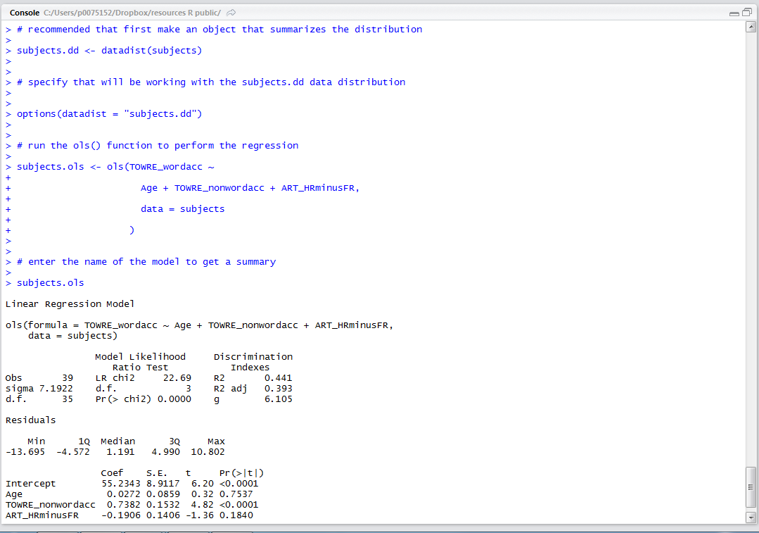
We then run the ols() function to produce our regression model of word reading skill for the ML lexical decision study participants. This function will run but not show us anything therefore we enter the model name to get a summary.

# recommended that first make an object that summarizes the distribution

subjects.dd <- datadist(subjects)

# specify that will be working with the subjects.dd data distribution

options(datadist = "subjects.dd")

# run the ols() function to perform the regression

subjects.ols <- ols(TOWRE_wordacc ~

 Age + TOWRE_nonwordacc + ART_HRminusFR,

 data = subjects

 )

# enter the name of the model to get a summary

subjects.ols

Look closely at what the R console will show you when you run this code:

Notice:

— When you run the model, you are entering a formula akin to the statistical form language you would use to specify a linear regression model.

— You enter:

subjects.ols <- ols(TOWRE_wordacc ~ Age + TOWRE_nonwordacc + ART_HRminusFR, data = subjects)

— A regression model might be written as:

— I can break the function call down:

subjects.ols —  the name of the model to be created

<- ols() — the model function call

TOWRE_wordacc — the dependent or outcome variable

~ — is predicted by

Age + TOWRE_nonwordacc + ART_HRminusFR — the predictors

, data = subjects — the specification of what dataframe will be used

— Notice also that when you run the model, you get nothing except the model command being repeated (and no error message if this is done right).

— To get the summary of the model, you need to enter the model name:

subjects.ols

— Notice when you look at the summary the following features:

Obs — the number of observations

d.f. — residual degrees of freedom

Sigma — the residual standard error i.e. the variability in model residuals — models that better fit the data would be associated with smaller spread of model errors (residuals)

Residuals — the listed residuals quartiles, an indication of the distribution of model errors — linear regression assumes that model errors are random, and that they are therefore distributed in a normal distribution

Model Likelihood Ratio Test — a measure of goodness of fit, with the test statistic, degrees of freedom (model predictors) and p-value reported

and — measures of the proportion of variance explained by the model.

In estimating the outcome (here, word reading skill), we are predicting the outcome given what we know about the predictors. Most of the time, the prediction will be imperfect, the predicted outcome will diverge from the observed outcome values. How closely do predicted values correspond to observed values? In other words, how far is the outcome independent of the predictor? Or, how much does the way in which values of the outcome vary coincide with the way in which values of the predictor vary? (I am paraphrasing Cohen et al., 2003, here.)

Let’s call the outcome Y and the predictor X. How much does the way in which the values of Y vary coincide with the way in which values of X vary? We are talking about variability, and that is typically measured in terms of the standard deviation SD or its square the variance . Variances are additive while SDs are not so we typically work with variances. In asking the string of questions given in the foregoing paragraph, we are thinking about a problem that can be expressed like this: what part of Y variance is associated with X (this part will equal the variance of the estimated scores) and what part of Y variance is independent of X (the model error, equal to the variance of the discrepancies between estimated and observed Y)? If there is no relationship between X and Y, our best estimate of Y will be the mean of Y. is the proportion of Y variance associated with X – our predictors.

Coef — a table presenting the model estimates for the effects of each predictor, while taking into account all other predictors

Notice:

— The estimated regression coefficients represent the rate of change in outcome units per unit change in the predictor variable.

— You could multiple the coefficient by a value for the predictor to get an estimate of the outcome for that value e.g. word reading skill is higher by 0.7382 times each unit increase in nonword reading score.

— The intercept (the regression constant or Y intercept) represents the estimated outcome when the predictors are equal to zero – you could say, the average outcome value assuming the predictors have no effect, here, a word reading score of 55.

For some problems, it is convenient to center the predictor variables by subtracting a variable’s mean value from each of its values. This can help alleviate nonessential collinearity (see here) due to scaling, when working with curvilinear effects terms and interactions, especially (Cohen et al., 2003). If both the outcome and predictor variables have been centered then the intercept will also equal zero. If just the predictor variable is centered then the intercept will equal the mean value for the outcome variable. Where there is no meaningful zero for a predictor (e.g. with age) centering predictors can help the interpretation of results. The slopes of the effects of the predictors are unaffected by centering.

— In addition to the coefficients, we also have values for each estimate for:

S.E. — the standard error of the estimated coefficient of the effect of the predictor. Imagine that we sampled our population many times and estimated the effect each time: those estimates would constitute a sampling distribution for the effect estimate coefficient, and would be approximately normally distributed. The spread of those estimates is given by the SE of the coefficients, which can be calculated in terms of the portion of variance not explained by the model along with the SDs of Y and of X.

t — the t statistic associated with the Null Hypothesis Significance Test (NHST, but see Cohen, 1994) that the effect of the predictor is actually zero. We assume that there is no effect of the predictor. We have an estimate of the possible spread of coefficient estimate values, given repeated sampling from the population, and reruns of the regression – that is given by the SE of the coefficient. The t-test in general is given by:

therefore, for regression coefficients:

i.e. for a null hypothesis that the coefficient should be zero, we divide the estimate of the coefficient, B, by the standard error of possible coefficients, to get a t-statistic

Pr(>|t|) — we can then get the probability that a value of t this large or larger by reference to the distribution of t values for the degrees of freedom at hand.

[I am skating over a whole bunch of stuff here but will return to each piece, in time.]

Assumptions

When we compute and discuss the correlation or regression and their coefficients to describe a sample of data, we do not need to make any assumptions. But most of the time, we want to infer something about a population given the sample. Cohen et al. (2003) note that the X and Y variables are distinguished as X an independent variable and Y a dependent variable, and that values of X are treated as fixed – we will see that term again when we move onto mixed-effects modelling – values of X are fixed in the sense that they are treated as if selected rather than sampled from the population. We look on the outcome, Y, as a sample from the population of possible values, so that for each value of X we might see a sample of Y values. We assume that the values of the discrepancy or difference or residual or error indicating the distance between our estimate of Y for any value of X, and the observed Y, is normally distributed in the population, and, in addition, that residuals have equal variances across values of X. These assumptions allow us to infer things about the population from the sample but we are not obliged to assume anything about the distribution of the X or of Y, nor about the sample itself.

What have we learnt?

(The code for running this analysis can be found here.)

Too much or not enough?

We have revised the computation and display of pairwise correlation coefficients.

We have then performed an ordinary least squares regression analysis.

We have added some notes on the analysis but we will revisit key concepts in time.

Key vocabulary

ols()

Reading

Baayen, R. H. (2008). Analyzing linguistic data. Cambridge University Press.
Castles, A., & Nation, K. (2006). How does orthographic learning happen? In S. Andrews (Ed.), From inkmarks to ideas: Challenges and controversies about word recognition and reading. Psychology Press.
Cohen, J., Cohen, P., West, S. G., & Aiken, L. S. (2003). Applied multiple regression/correlation analysis for the behavioural sciences (3rd. edition). Mahwah, NJ: Lawrence Erlbaum Associates.
Harm, M. W., & Seidenberg, M. S. (2004). Computing the meanings of words in reading: Cooperative division of labor between visual and phonological processes. Psychological Review, 111, 662-720.
Harrell Jr, F. J. (2001). Regression modelling strategies: With applications to linear models, logistic regression, survival analysis. New York, NY: Springer.
Masterson, J., & Hayes, M. (2007). Development and data for UK versions of an author and title recognition test for adults. Journal of Research in Reading, 30, 212-219.
Nation, K. (2008). Learning to read words. The Quarterly Journal of Experimental Psychology, 61, 1121-1133.
Rayner, K., Foorman, B. R., Perfetti, C. A., Pesetsky, D., & Seidenberg, M. S. (2001). How psychological science informs the teaching of reading. Psychological Science in the Public Interest, 2, 31-74.
Share, D. L. (1995). Phonological recoding and self-teaching: sine qua non of reading acquisition. Cognition, 55, 151-218.
Stanovich, K. E., & West, R. F. (1989). Exposure to print and orthographic processing. Reading Research Quarterly, 24, 402-433.
Torgesen, J. K., Wagner, R. K., & Rashotte, C. A. (1999). TOWRE Test of word reading efficiency. Austin,TX: Pro-ed.