This post will build on the previous Modelling posts. We are continuing to focus on the item norms data, previously discussed here and here (where I talked about were the data are from), here and here (where I talked about examining the distribution of variables like length) and here (where I talked about examining the relationships between pairs of variables.

I want to move on to examine the relationships between the variables corresponding to a larger set of item attributes than just the length, orthographic neighbourhood size and bigram frequency of items. The latter variables are measures that apply to words as well as to nonwords. I want to bring in variables capturing also, for each word: how common it is in our experience (frequency); how early in life we learnt it (age-of-acquisition, AoA); and how easy it is to imagine the referent or concept that the word names (imageability). There is an extensive literature on why these variables might be considered influential in an examination of variation in reading performance; interested readers can start with the recent papers examining the effects of these variables on observed reading behaviour (Adelman, Brown & Quesada, 2009; Balota et al., 2004;  Brysbaert & New, 2010; Cortese & Khanna, 2007).

We have data on the frequency, AoA and imageability measures in one data base, and on length, neighbourhood and bigram frequency in another.

The purpose of this post is to show how to put the databases together, and then modify them for our purposes.

Download the datafiles and read them into the workspace

As shown previously, we start by downloading the databases required:

We have .csv files holding:

1. data on the words and nonwords, variables common to both like word length;

2. data on word and nonword item coding, corresponding to item in program information, that will allow us to link these norms data to data collected during the lexical decision task;

3. data on just the words, e.g. age-of-acquisition, which obviously do not obtain for the nonwords.

Click on the links to download the files, then read them into the workspace using read(), as shown here.

We will be focusing on the dataframes:

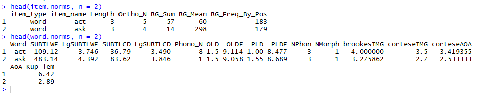
item.norms

word.norms

There are 160 words and 160 nonwords in the items dataframe. The same 160 words are in the words dataframe. Critically,  the words are listed by name in the item_type column in item.norms and in the Word column in word.norms.

We can use this common information as an index to merge the item and word norms data.

Rename variables

To merge two dataframes, there needs to be a common index in both. We have that common index but it has different names in the different dataframes. We solve this problem by renaming one of the variables using the rename() function from the reshape() package.

word.norms <- rename(word.norms, c(Word = "item_name"))

Notice:

— We are recreating the word.norms database from itself, with the rename() function call transforming the name of that name variable, capital W word.

— Don’t ask me why you need to put the old and the new column names in a c() concatenate function, I guess you might consider the pair of names to be a vector with two elements.

If you run that line of code, the renaming is done. Easy

Check that the word names in the item_name column in each dataframe do match

Before we can merge the dataframes by the common index of word names, now item_name, we need to check that the columns do have all item word names in common.

As mentioned, there are 160 words in each dataframe. Name is, of course, a nominal variable, a factor. We can inspect the levels (here, the different names) in a factor using the levels() function.

levels(item.norms$item_name)

levels(word.norms$item_name)

Which will show you this:

Can you see the problem?

The word false is “FALSE” in word.norms and in item.norms. Sometimes, you have “false” in one dataframe and “FALSE” in another. All this false-FALSE happened because some of the .csv files were prepared in excel and in excel false or true automatically get converted to FALSE and TRUE because they are words that are reserved to refer to logic values. If we merge two dataframes with “false” in one but “FALSE” in the other, this difference in case would count as a mismatch because “false” is not == to “FALSE”.

Read the R help on merge here. It is a powerful and useful function, well worth the effort.

However, you have to be careful.

In merge():

1. R examines the common columns in the two dataframes. I imagine a logical test is done, row by row: do the rows match on the common column, TRUE or FALSE?

2. The rows in the two data frames that do match on the specified columns are extracted, and joined together.

N.B. If there is more than one match, all possible matches contribute one row each. This can lead to you getting more rows than expected in the output dataframe from merger, i.e. some kind of row duplication occurs.

N.B. You can merge dataframes on the basis of more than one common index.

Any mismatch causes a problem when we try to merge the dataframes because observations pertaining to the mismatch index entry will simply be dropped.

In merging item.norms and word.norms the resulting dataframe will not include data on the nonwords simply because there is no match for the latter in the word.norms dataframe.

The merge() operation does not require the rows to be sorted or to occur in the same order.

Merge dataframes by the common variable item_name

Now we have two dataframes with a common index of item names, with all names matching at least for words, we can do the merger as follows:

# now can merge the two norms databases

item.words.norms <- merge(item.norms, word.norms, by = "item_name")

# and inspect the results

head(item.words.norms, n = 2)
summary(item.words.norms)
describe(item.words.norms)
str(item.words.norms)
length(item.words.norms)
length(item.words.norms$item_name)
levels(item.word.norms$item_name)

When we inspect the results, things look as expected – an important sanity check – as we can see by considering the results of the summary() call.

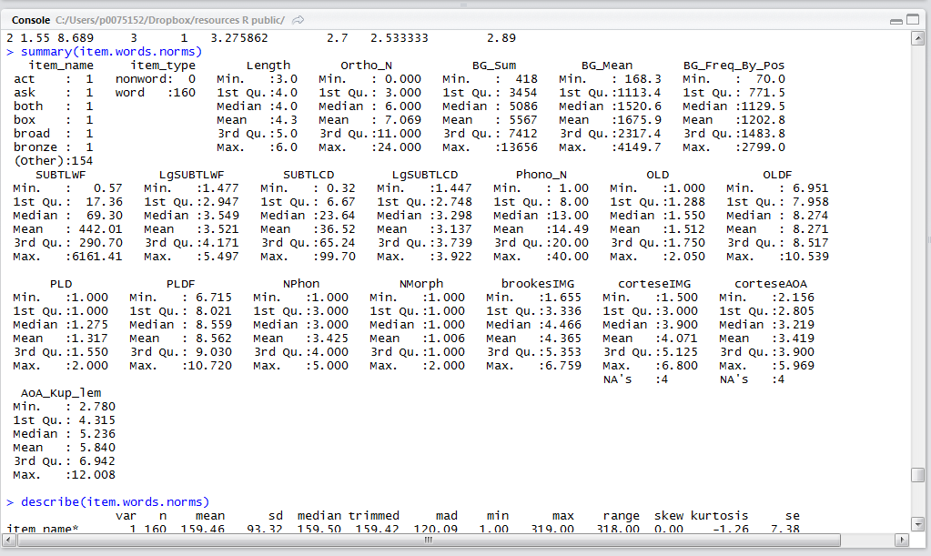
Notice:

— We have 160 words and no nonwords in the new dataframe.

— We have both the items and the words data in the same dataframe.

— There are a bunch of missing values on the Cortese variables – where some words did not have values in those databases for those variables.

— Those missings led me to collect some imageability ratings (brookesIMG) and get the Kuperman AoA values for these words.

Create a csv file from this dataframe resulting from our various transform, rename, merge operations

Just as one can read.csv() an excel readable .csv file, one can output or write a .csv file.

I do not want to go through all the things I have done again, so I create a file out of the result of all these operations. N.B. I think I found out how to do this in Paul Teetor’s (2011) “R cookbook” but I also think the advice is, as usual, all over the web.

# we can write this dbase out to csv:

write.csv(item.words.norms, file = "item.words.norms 050513.csv", row.names = FALSE)

The csv file will then be found in your working directory.

Check it out, compare it to the original component word.norms and item.norms csv files.

What have we learnt?

(The code to run this data merger can be found here.)

We have learnt to rename a dataframe variable.

We have learnt to inspect then merge two dataframes on the basis of a common variable, here, an item name index.

We have learnt how to output the resulting dataframe as a .csv file.

Key vocabulary

rename()

levels()

merge()

write.csv()

Reading

Adelman, J. S., Brown, G. D. A., & Quesada, J. F. (2006). Contextual diversity not frequency determines word naming and lexical decision times. Psychological Science, 17 814-823.
Balota, D., Cortese, M. J., Sergent-Marshall, S. D., Spieler, D., & Yap, M. (2004). Visual word recognition of single-syllable words. Journal of Experimental Psychology: General, 133, 283-316.
Brysbaert, M., & New, B. (2009). Moving beyond Kucera and Francis: A critical evaluation of current word frequency norms and the introduction of a new and improved frequency measure for American English. Behavior Research Methods, 41(4), 977-990.
Cortese, M. J., & Khanna, M. M. (2007). Age of acquisition predicts naming and lexical-decision performance above and beyond 22 other predictor variables: An analysis of 2,342 words. The Quarterly Journal of Experimental Psychology, 60, 1072-1082.