This post follows on from the previous post, concerning the examination of variable distributions.

It is always useful to plot the distribution of variables like item attributes e.g. item length in letters. One important benefit of doing so is identifying whether your dataset is in the shape you expect it to be in: identifying errors, of input or coding, should happen early in analysis so I urge you to plot and examine the plots of your data as soon as you get started.

However, psycholinguistics papers typically report stimulus characteristics in the form of a tabled summary of the means and SDs of the attributes of your stimuli, possibly broken down by item type (e.g. words vs. nonwords). In addition, reports of stimuli typically include the results of comparisons of the mean values of item attributes for each stimulus item type.

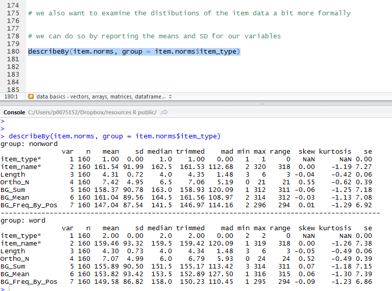
We can get the summary statistics for our item attribute variables using the handy psych package function describeBy(). In making that function call, we specify that we want the item norms data statistics split by item type. The R output can be converted into a table in a number of different ways. The easiest elegant method would be to writing your report in knitr all inside R-studio. The easiest horrible method, for someone writing a report in Microsoft Word, would be to paste the R output in a .txt document, open that document in excel, sort the formatting of the table out in excel, paste that table into Word as a bitmap. I use the horrible method all the time, because I haven’t yet learnt how to knit in R, though I will, because the horrible method is horrible.

Reporting the mean length etc. of the words and nonwords will not be enough. We also need to test the difference between the mean lengths etc. of the words and nonwords statistically. We can do this using the t-test, so long as the data distributions are ‘reasonably’ normal; if they are not, we might prefer to use non-parametric tests to compare means.

I am not going to get into the theory behind the t-test here, though I wrote a set of slides for  an undergraduate statistics class which can be accessed at this link.

https://speakerdeck.com/robayedavies/t-test

I recommend reading Howell (2002) if you are unsure about t-tests. I have never found a clearer exposition of the logic of the main statistical tests (except maybe in Jacob Cohen’s writings).

I will come back to this important and pervasive test statistic in another post.

The code that we use to both get the summary statistics and perform the t-tests is very concise.

describeBy(item.norms, group = item.norms$item_type)

will get you a table of all the summary statistics you might need:

And we can test the difference between the mean values for words vs. nonwords on each item variable as follows:

t.test(Length ~ item_type, data = item.norms)
t.test(Ortho_N ~ item_type, data = item.norms)
t.test(BG_Sum ~ item_type, data = item.norms)
t.test(BG_Mean ~ item_type, data = item.norms)
t.test(BG_Freq_By_Pos ~ item_type, data = item.norms)

which will give us a series of results (output fragment – screenshot shown):

telling us that words and nonwords are not significantly different on mean length, orthographic neighbourhood size or any of the bigram frequency measures.

What have we learnt?

(The code for doing these statistics can be found here.)

It is very easy to statistically describe and then examine the distribution of variables in R.

Key vocabulary

describeBy()

t.test()

Reading

Howell, D. C. (2002). Statistical methods for psychology (5th. Edition). Pacific Grove, CA: Duxbury.