
I am going to take another shot at considering mixed effects modelling. This time from a perspective closer to my starting point. I first learnt about mixed-effects modelling through reading about it in, I think, some paper or chapter by Harald Baayen in the mid-2000s (maybe, Baayen et al., 2002). In 2007, I attended a seminar by Marc Brysbaert on ‘The Language as fixed-effect fallacy’ which ended in a recommendation to consider mixed-effects modelling and to try lmer in R. The workshop title is a reference to a highly influential paper by Clark (1973; see, also, Raaijmakers et al., 1999) and a familiar problem for many psycholinguists.
The problem is this:
I might have an expectation about some language behaviour, for example, that words appearing often in the language are easier to read, or that word choice in speaking is mediated through a process of selection by competition. I perform an experiment in which I test some number of individuals (let’s say, 20) with some number of stimuli (let’s say 20). Perhaps the stimuli vary in frequency, or perhaps I present them in two conditions (say, once superimposed on pictures of semantically related objects, once on pictures of unrelated objects). I do not really care who any one person is, I am mostly interested in the effect of frequency or semantic relatedness in general, and regard the specific characteristics of the people being tested as random variation, seeing the group of people being tested as a random sample from the population of readers or speakers. Likewise, I wish to infer something about language and would consider the particular words being presented as a random sample from the wider population of words. For both samples, I would wish to estimate the effect of interest to me while accounting for random variation in performance due to participant or item sampling.
Clark (1973) argued that to draw conclusions from data like these that might apply generally, one ought to analyze the data using an approach that took into account the random effects of both participants and individuals. As I noted previously, if you look at data on a participant-by-participant basis, you will find ample evidence for both variation across individuals about some average effect and variation across items about some average effect.
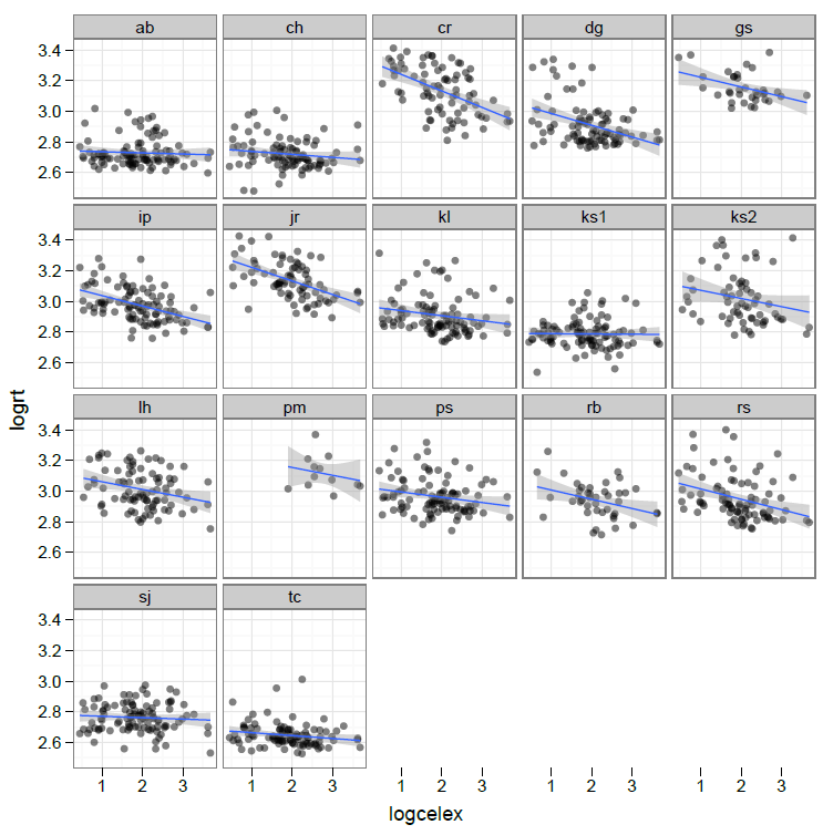
Individual differences – adults reading aloud, 100 words, English – RT by log frequency
Around 2006, I was conducting a regression analysis of Spanish reading data and finding quite big variation in the size and sometimes the direction of effects across individuals all of whom had been presented with the same words under the same circumstances.
Now, if you look at Clark’s (1973) paper, you can see him consider what researchers at the time did and what they should do about subject and item random effects. Conventionally, one had averaged across responses to the different words for each participant to get an average RT by-subjects per condition, ignoring variation between items (the fact that the items were sampled from a wider population) and thus inflating the possibility that an effect is spuriously detected when it is not present. The key difficulty is to estimate error variance appropriately. One is seeking to establish if variance due to an effect is greater than variance due to error variation, but this will only guide us correctly if the error variance includes both error variance due to subject and that due to item sampling. Clark (1973) recommended calculating F’, the quasi F-ratio, as the ratio of the variance due to the effect compared to the variance due to variance (in the effect) due to random variation between subjects or items. As a shortcut to the needed analysis, Clark (1973) suggested one could perform an analysis of the effect as it varied by subjects and an analysis of the effect as it varied by items. Conventionally, this subsequently meant that one could average over responses to different items for each person to get the average responses by-subjects and perform a by-subjects ANOVA (F1) or t-test (t1), and one could also average over responses by different people to each item to get the average responses by-items and perform a by-items ANOVA (F2) or t-test (t2). Using a very simple formula, one could then form minF’ as the ratio:

and then more accurately estimate the effect with respect to the null hypothesis taking into account both subject and item random effects.
Not simple enough, as Raaijmakers et al. (1999) report, psychologists soon stopped calculating minF’ and resorted just to reporting F1 and F2 separately or (informally) together. It has been quite typical to refer to an effect that is significant in F1 and F2 as significant but Raaijmakers et al. (1999) show that even if F1 + F2 are significant that does not mean that minF’ will be.
I spent a bit of time calculating minF’ and, if I were doing ANOVA and not lmer, I would do it still (see Baayen et al., 2008, for an analysis of how well minF’ does in terms of both Type I and II errors).
That is fine. But what if you’re doing a reading experiment in which you are concerned about the effects on reading of item attributes and you have read Cohen (1983) or his other commentary on the cost of dichotomizing continous variables? What you would not do is present items selected to conform to the manipulation of some factor e.g. selecting items that were low in frequency or high in frequency (but matched on everything else) to test the effect of frequency on reading. This is because in performing a factorial study like that, essentially, cutting a continuous variable (like frequency) into two, one is reducing the capacity of the analysis to detect an effect that really is there (increasing the Type II error rate), as Cohen (1983) explained. What you would do, then, is to perform a regression analysis. In most circumstances, one might present a large-ish set of words to a sample of participants, giving each person the same words so that the study take a repeated-measures approach. One can then average over subjects for each word to get the average by-items reaction times (or proportion of responses correct) and then perform an analysis of the manner in which reading performance is affected by an item attribute like frequency.
However, Lorch & Myer (1990) pointed out that if you performed by-items regressions on repeated measures data then you would be vulnerable to the effect of making subjects a fixed effect: effects might be found to be significant simply because of variation over subjects in the effect of the item attribute. They recommend a few alternatives. One is to not average data over subjects but arrange the raw observations (one RT corresponding to a person’s response to a word) in a long format database then perform a regression in which: 1. item attributes are predictors (in long format, one would have to copy item attribute data for each person’s observations); 2. subject identity is coded using dummy coding variables (with n subjects – 1 columns). Another approach is to perform a regression analysis for each person’s data individually, then conduct a further test (e.g. a one-sample t-test) of whether a vector of the per-person regression coefficients for an effect is significantly different from zero. Balota et al. (2004) take the latter approach.
But you can see the potential problems if you look at the lattice of individual data plots above, and at the following plot from an old study of mine:
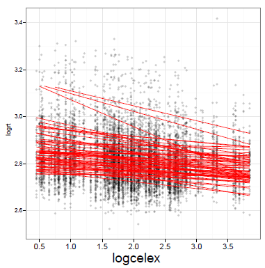
60 children, aged 10-12 years, logRT reading aloud by logcelex frequency
What you can see is the effect of frequency on the performance of each individual reader, estimated in a per-individual regression analysis.
Notice:
— Variation in the intercept i.e. the average RT per person.
— Variation in the slope of the effect.
If you think about it, and look at some of the low-scoring participants in the lattice plot, above, you can also see that the size of the sample of observations available for each person will also vary. Doing a t-test on effects coefficients calculated for each individual will not allow you to take into account the variation in reliability of that effect over the sample.
As Baayen et al. (2008) point out, it turns out that both the by-items regressions and by-subjects regression approaches have problems accounting properly for random effects due to subjects and to items (with departures from the nominal error rate i.e. p does not necessarily = 0.05 when these analyses say it does), and may suffer from restricted sensitivity to effects that really are present.
It is at that point, that I turned to mixed-effects modelling.
Reading
Baayen, R. H., Davidson, D. J., & Bates, D. M. (2008). Mixed-effects modeling with crossed random effects for subjects and items. Journal of Memory and Language, 59, 390-412.
Baayen, R. H., Tweedie, F. J., & Schreuder, R. (2002). The subjects as a simple random effect fallacy: Subject variability and morphological family effects in the mental lexicon. Brain and Language, 81, 55-65.
Balota, D., Cortese, M. J., Sergent-Marshall, S. D., Spieler, D., & Yap, M. (2004). Visual word recognition of single-syllable words. Journal of Experimental Psychology: General, 133, 283-316.
Brysbaert, M. (2008). “The language-as-fixed-effect fallacy”: Some simple SPSS solutions to a complex problem.
Clark, H. H. (1973). The language-as-fixed-effect fallacy: A critique of language statistics in psychological science. Journal of Verbal Learning and Verbal Behaviour, 12, 335-359.
Cohen, J. (1983). The cost of dichotomization. Applied Psychological Measurement, 7, 249-253.
Lorch, R. F., & Myers, J. L. (1990). Regression Analyses of Repeated Measures Data in Cognitive Research. Journal of Experimental Psychology: Learning, Memory and Cognition, 16(1), 149-157.
Raaijmakers, J. G. W., Schrijnemakers, J. M. C., & Gremmen, F. (1999). How to deal with the “Language-as-fixed-effect Fallacy”: Common misconceptions and alternative solutions. Journal of Memory and Language, 41, 416-426.
