
In the last post, I showed how to collate the various data bases we constructed or collated from the data collection achieved in a study of lexical decision. We ended the post by producing a .csv file of the output of our various merger operations, which can be downloaded here.
This file holds data on:
1. participant attributes;
2. word attributes;
3. participant responses to words in the lexical decision task.
In this post, I want to take a quick look at how you would actually run a mixed-effects model, using the lmer() function furnished by the lme4 package, written by Doug Bates (Bates, 2010 – appears to a preprint of his presumed new book, see also Pinheiro & Bates, 2000). A useful how-to guide, one I followed when I first started doing this kind of modelling, is in Baayen (2008). An excellent, and very highly cited, introduction to mixed-effects modelling for psycholinguistics, is found in Baayen, Davidson & Bates (2008).

First, then, we enter the following lines of code to load the libraries we are likely to need, to set the working directory to the folder where we have copied the full database, and to read that database as a dataframe in the session’s workspace:
library(languageR)
library(lme4)
library(ggplot2)
library(grid)
library(rms)
library(plyr)
library(reshape2)
library(psych)
library(gridExtra)

# set the working directory

setwd("C:/Users/p0075152/Dropbox/resources R public")

# read in the full database

item.words.norms <- read.csv("RTs.norms.subjects 090513.csv", header=T, na.strings = "-999")
We should then inspect what we get:
# inspect the dataframe

head(RTs.norms.subjects, n = 2)
summary(RTs.norms.subjects)
describe(RTs.norms.subjects)
str(RTs.norms.subjects)
length(RTs.norms.subjects)
length(RTs.norms.subjects$item_name)
levels(RTs.norms.subjects$item_name)
If we consider the output from the summary() function call, we can see mostly what we expect and one thing we need to deal with before we do any modelling:
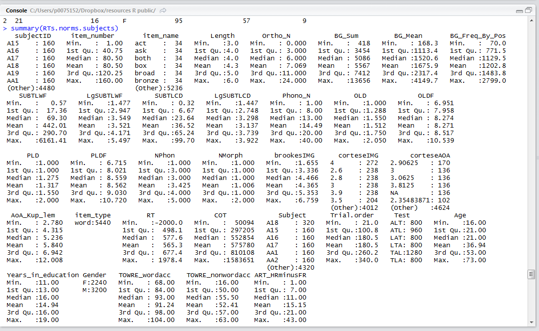
Notice:
— The minimum value for the RT variable is -2000. Negative RTs arise because DMDX will record a correct response as a positive and an incorrect response as a negative number, and we did not deal with that fact through the whole data collation process.
In fact, having incorrect responses associated with negative RTs is useful because we can subset the dataframe, setting a condition on rows, to remove all observations pertaining to errors.
nomissing.full <- RTs.norms.subjects[RTs.norms.subjects$RT > 0,]

summary(nomissing.full)
You will see, if you run those lines, that the summary of the new no missing i.e. no errors dataframe has 5257 rows, the ones we lost are the errors, as we can see that the minimum RT is now 262.2 (might be worth considering if that RT is too small, a recording error, another time).
We can then move on to run the mixed-effects model:
full.lmer1 <- lmer(RT ~
 Trial.order +

 Age + TOWRE_wordacc + TOWRE_nonwordacc + ART_HRminusFR +

 Length + OLD + BG_Mean + LgSUBTLCD + AoA_Kup_lem + brookesIMG +

 (1|subjectID) + (1|item_name),

 data = nomissing.full)

print(full.lmer1,corr=F)
Notice:
— We are running the model using the lmer() function.
— We specify that the dataframe in play is the nomissing.full one we just created.
— We created a model, the object assigned to a name full.lmer1, with the lmer() function call.
— We later output a summary of that model using the print() function call; no output would be shown otherwise.
— The model has the following components:
1. RT — the outcome or dependent variable
2. ~ — predicted by
3. A set of predictors including:
Trial.order +
Age + TOWRE_wordacc + TOWRE_nonwordacc + ART_HRminusFR +
Length + OLD + BG_Mean + LgSUBTLCD + AoA_Kup_lem + brookesIMG +
— the fixed effects.
4. A set of predictors also including:
(1|subjectID) + (1|item_name)
— the random effects, here, random effects due to participant and item effects on intercepts.
The output summary of this model is shown in the R-studio console window as:
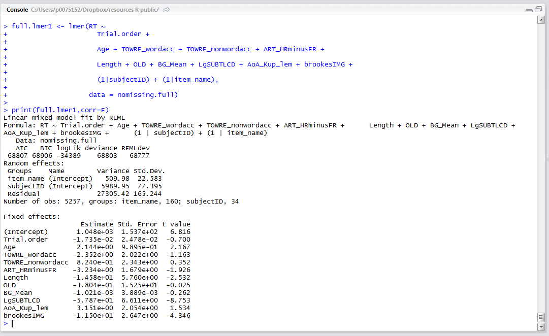
Notice:
— We do not get p-values.
— We are shown the estimated spread of random effects.
— We are shown the fixed effects in a format equivalent to the coefficients summary table for a regression analysis.
— Knowing that if 
1. Age — older readers had slower RTs;
2. ART score — more experienced readers were faster;
3. Length — longer words elicited shorter RTs;
4. Frequency – LgSUBTLCD — more frequent words elicited shorter RTs;
5. Imageability – IMG – more imageable words elicited shorter RTs.
Aside from the length effect which contrasts with some previous reports (Weeks, 1997) but not others (New et al., 2007), these effects are consistent with numerous previous observations in the literature.
We could take these results to a report, if we wanted.
Obviously, however, what we will do in later posts will be to consider how we can examine and display the utility and the validity of this model, and models like it.
What have we learnt?
(The code used to run the model can be found here.)
Well, not much, just how to run a lmer() mixed-effects model. The real work is just starting.
Key vocabulary
lmer()
Reading
Baayen, R. H. (2008). Analyzing linguistic data. Cambridge University Press.
Baayen, R. H., Davidson, D. J., & Bates, D. M. (2008). Mixed-effects modeling with crossed random effects for subjects and items. Journal of Memory and Language, 59, 390-412.
Balota, D., Cortese, M. J., Sergent-Marshall, S. D., Spieler, D., & Yap, M. (2004). Visual word recognition of single-syllable words. Journal of Experimental Psychology: General, 133, 283-316.
Bates, D. M. (2005). Fitting linear mixed models in R. R News, 5, 27-30.
New, B., Ferrand, L., Pallier, C., & Brysbaert, M. (2007). Re-examining the word length effect in visual word recognition: New evidence from the English lexicon project. Psychonomic Bulletin and Review, in press
Pinheiro, J. C., & Bates, D. M. (2000). Mixed-effects models in S and S-plus (Statistics and Computing). New York: Springer.
Weekes, B. S. (1997). Differential effects of number of letters on word and nonword naming latency. The Quarterly Journal Of Experimental Psychology, 510A 439-456.
