
We completed a study on the factors that influence visual word recognition performance in lexical decision. We then put together a dataset for analysis here. We examined the distribution of inter-relation of critical variables in that dataset, acting to transform the data where we found indications of concern, here.
We will now proceed to analyse the lexical decision reaction times (RTs). The dataset collated in the last post consisted of observations corresponding to correct responses to words only, RTs along with data about the subject and item attributes. It will be recalled that we wish to examine the effects on reading of who is reading and what they are reading.
The last collated dataset can be downloaded here.
The code I am going to use in this post can be downloaded here.
We are going to start by ignoring the random effects structure of the data, i.e. the fact that the data are collected in a repeated measures design where every participant saw every word so that there are dependencies between observations made by each participant (some people are slower than others, and most of their responses will be slower) and dependencies between observations made to each item (some words are harder than others, and will be found to be harder by most readers). What we will do is perform Ordinary Least Squares (OLS) regression with our data, and drawing scatterplots will be quite central to our work (see previous posts here and here). I am going to assume familiarity with correlation and OLS regression (but see previous posts here and here).
The relationships between pairs of variables — scatterplots
We are interested in whether our readers are recognizing some words faster than others. Previous research (e.g. Balota et al., 2004) might lead us to expect that they should respond faster to more frequent, shorter, words that are easier to imagine (the referent of). We are also interested in whether individuals vary in how they recognize words. We might expect that readers who score high on standardized reading tests (e.g. the TOWRE) would also respond faster, on average, in the experimental reading task (lexical decision). The interesting question, for me, is whether there is an interaction between the first set of effects — of what is being read — and the second set of effects — who is doing the reading.
We have already looked at plots illustrating the relationships between various sets of the predictor variables: scatterplot matrices.
We are now going to create a trellis of scatterplots to examine the relationship between each predictor variable and word recognition RT.
Let’s start with a scatterplot. I assume the collated dataset has been downloaded and is available for use in R’s workspace. If you copy the following code to draw a plot:
plength <- ggplot(nomissing.full,aes(x=Length, y=RT))
plength <- plength + geom_jitter(colour = "black", alpha = 1/5)
plength <- plength + xlab("Length") + theme_bw()
plength <- plength + theme(axis.title.x = element_text(size=25)) + theme(axis.text.x = element_text(size=20))
plength <- plength + geom_smooth(method="lm", size = 1.5)
plength
You will get this:
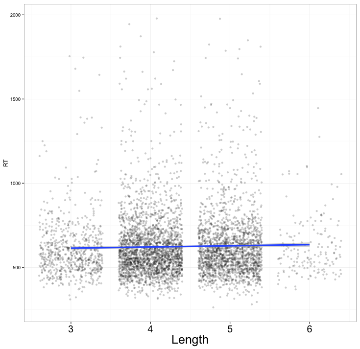
Notice:
– I am adding each element, one at a time, making for more lines of code but greater transparency between code and effect.
— I first ask to have a plot object created: plength <- ggplot(nomissing.full,aes(x=Length, y=RT))
— the object is called plength, the function doing the creation is ggplot(), it is acting on the database nomissing.full, and it will map the variables Length to x coordinate and RT to y coordinate
— the mapping is from data to aesthetic attributes like point location in a scatterplot
— I then add to what is a blank plot the geometric object (geom) point — run the first line alone and see what happens
— here I am asking for jittered points with + geom_jitter(colour = “black”, alpha = 1/5) — where a bit of random noise has been added to the point locations because so many would otherwise appear in the same place — overplotting that obscures the pattern of interest — I am also modifying the relative opacity of the points with alpha = 1/5
– I could add the scatterplot points with: + geom_point() —
substitute that in for geom_jitter() and see what happens — I could change the colour scheme also
– I then change the axis label with: + xlab(“Length”)
– I modify the size of the labeling with: + theme(axis.title.x = element_text(size=25)) + theme(axis.text.x = element_text(size=20))
– I add a smoother i.e. a line showing a linear model prediction of y-axis values for the x-axis variable values with: + geom_smooth(method=”lm”, size = 1.5) – and I ask for the size to be increased for better readability
– and I ask for the plot to have a white background with: + theme_bw()
In fact, I would like to see a plot of all the key predictor variables and their effect on RT, considering just the bivariate relationships. It is relatively easy to first draw each plot, then create a trellis of plots, as follows:
# 1. are RTs affected by item attributes?

# let's look at the way in which RT relates to the word attributes, picking the most obvious variables
# we will focus, here, on the database holding correct responses to words

head(nomissing.full, n = 2)

plength <- ggplot(nomissing.full,aes(x=Length, y=RT))
plength <- plength + geom_jitter(colour = "black", alpha = 1/5)
plength <- plength + xlab("Length") + theme_bw()
plength <- plength + theme(axis.title.x = element_text(size=25)) + theme(axis.text.x = element_text(size=20))
plength <- plength + geom_smooth(method="lm", size = 1.5)
plength

pOLD <- ggplot(nomissing.full,aes(x=OLD, y=RT))
pOLD <- pOLD + geom_jitter(colour = "black", alpha = 1/5)
pOLD <- pOLD + xlab("OLD") + theme_bw()
pOLD <- pOLD + theme(axis.title.x = element_text(size=25)) + theme(axis.text.x = element_text(size=20))
pOLD <- pOLD + geom_smooth(method="lm", size = 1.5)
pOLD

pfreq <- ggplot(nomissing.full,aes(x=LgSUBTLCD, y=RT))
pfreq <- pfreq + geom_point(colour = "black", alpha = 1/5)
pfreq <- pfreq + xlab("LgSUBTLCD") + theme_bw()
pfreq <- pfreq + theme(axis.title.x = element_text(size=25)) + theme(axis.text.x = element_text(size=20))
pfreq <- pfreq + geom_smooth(method="lm", size = 1.5)
pfreq

pAoA_Kup_lem <- ggplot(nomissing.full,aes(x=AoA_Kup_lem, y=RT))
pAoA_Kup_lem <- pAoA_Kup_lem + geom_point(colour = "black", alpha = 1/5)
pAoA_Kup_lem <- pAoA_Kup_lem + xlab("AoA") + theme_bw()
pAoA_Kup_lem <- pAoA_Kup_lem + theme(axis.title.x = element_text(size=25)) + theme(axis.text.x = element_text(size=20))
pAoA_Kup_lem <- pAoA_Kup_lem + geom_smooth(method="lm", size = 1.5)
pAoA_Kup_lem

pbrookesIMG <- ggplot(nomissing.full,aes(x=brookesIMG, y=RT))
pbrookesIMG <- pbrookesIMG + geom_jitter(colour = "black", alpha = 1/5)
pbrookesIMG <- pbrookesIMG + xlab("Imageability") + theme_bw()
pbrookesIMG <- pbrookesIMG + theme(axis.title.x = element_text(size=25)) + theme(axis.text.x = element_text(size=20))
pbrookesIMG <- pbrookesIMG + geom_smooth(method="lm", size = 1.5)
pbrookesIMG

# 2. are RTs affected by subject attributes?

# let's look at the way in which RT relates to the word attributes, picking the most obvious variables
# we will focus, here, on the database holding correct responses to words

head(nomissing.full, n = 2)

pAge <- ggplot(nomissing.full,aes(x=Age, y=RT))
pAge <- pAge + geom_jitter(colour = "black", alpha = 1/5)
pAge <- pAge + xlab("Age") + theme_bw()
pAge <- pAge + theme(axis.title.x = element_text(size=25)) + theme(axis.text.x = element_text(size=20))
pAge <- pAge + geom_smooth(method="lm", size = 1.5)
pAge

pTOWRE_wordacc <- ggplot(nomissing.full,aes(x=TOWRE_wordacc, y=RT))
pTOWRE_wordacc <- pTOWRE_wordacc + geom_jitter(colour = "black", alpha = 1/5)
pTOWRE_wordacc <- pTOWRE_wordacc + xlab("TOWRE word") + theme_bw()
pTOWRE_wordacc <- pTOWRE_wordacc + theme(axis.title.x = element_text(size=25)) + theme(axis.text.x = element_text(size=20))
pTOWRE_wordacc <- pTOWRE_wordacc + geom_smooth(method="lm", size = 1.5)
pTOWRE_wordacc

pTOWRE_nonwordacc <- ggplot(nomissing.full,aes(x=TOWRE_nonwordacc, y=RT))
pTOWRE_nonwordacc <- pTOWRE_nonwordacc + geom_jitter(colour = "black", alpha = 1/5)
pTOWRE_nonwordacc <- pTOWRE_nonwordacc + xlab("TOWRE nonword") + theme_bw()
pTOWRE_nonwordacc <- pTOWRE_nonwordacc + theme(axis.title.x = element_text(size=25)) + theme(axis.text.x = element_text(size=20))
pTOWRE_nonwordacc <- pTOWRE_nonwordacc + geom_smooth(method="lm", size = 1.5)
pTOWRE_nonwordacc

pART_HRminusFR <- ggplot(nomissing.full,aes(x=ART_HRminusFR, y=RT))
pART_HRminusFR <- pART_HRminusFR + geom_jitter(colour = "black", alpha = 1/5)
pART_HRminusFR <- pART_HRminusFR + xlab("ART print exposure") + theme_bw()
pART_HRminusFR <- pART_HRminusFR + theme(axis.title.x = element_text(size=25)) + theme(axis.text.x = element_text(size=20))
pART_HRminusFR <- pART_HRminusFR + geom_smooth(method="lm", size = 1.5)
pART_HRminusFR
Notice:
— What is changing between plots are: plot object names, the x-axis variable name (spelled correctly) and plot x axis label
— You can run each set of code to examine the relationships between predictor variables and RT one at a time.
We can create a grid and then print the plots to specific locations in the grid, as follows, outputting everything as a pdf:
pdf("nomissing.full-RT-by-main-effects-subjects-061113.pdf", width = 18, height = 12)

grid.newpage()

pushViewport(viewport(layout = grid.layout(2,5)))

vplayout <- function(x,y)
viewport(layout.pos.row = x, layout.pos.col = y)

print(plength, vp = vplayout(1,1))
print(pOLD, vp = vplayout(1,2))
print(pfreq, vp = vplayout(1,3))
print(pAoA_Kup_lem, vp = vplayout(1,4))
print(pbrookesIMG, vp = vplayout(1,5))

print(pAge, vp = vplayout(2,1))
print(pTOWRE_wordacc, vp = vplayout(2,2))
print(pTOWRE_nonwordacc, vp = vplayout(2,3))
print(pART_HRminusFR, vp = vplayout(2,4))

dev.off()
If you run that code it will get you this:
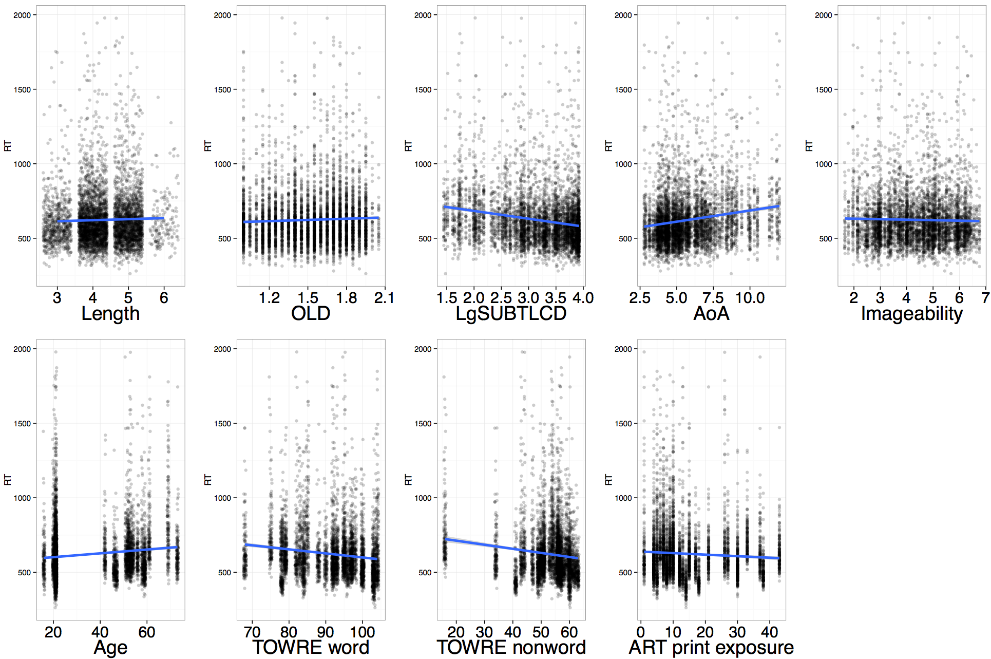
What is your evaluation?
The next question obviously is the extent to which these variables make unique contributions to the explanation of variance in reading RT, when taking the other variables into account, and whether we might detect interactions between effects of item attributes like frequency and person attributes like word reading skill.
We can examine potential interactions by splitting the data into subsets, effectively, through the creation of a variable that associates observations with intervals in one of the components of the potential interaction. In other words, if we wanted to look at the age x frequency interaction, we might look at the frequency effect for each of four subsets of the data, corresponding to four equal intervals in the age variable. We can use the following code to do that:
# first, add coding variables that split the dataset into equal intervals according to scores on each subject
# attribute of interest

nomissing.full$TOWRE_wordacc_cutequal <- cut_interval(nomissing.full$TOWRE_wordacc, n = 4)

#then plot the interaction: age x frequency

pdf("nomissing.full-freqwords-rt-lm-scatter-061113.pdf", width = 12, height = 8)

pLgSUBTLCD <- ggplot(nomissing.full,aes(x=LgSUBTLCD,y=RT))
pLgSUBTLCD <- pLgSUBTLCD + geom_jitter(colour = "black", alpha = 1/5) + theme_bw()+ xlab("LgSUBTLCD") # +
pLgSUBTLCD <- pLgSUBTLCD + theme(axis.title.x = element_text(size=25)) + theme(axis.text.x = element_text(size=10))
pLgSUBTLCD <- pLgSUBTLCD + geom_smooth(method="lm", size = 1.5, colour = "red")
pLgSUBTLCD <- pLgSUBTLCD + facet_wrap(~TOWRE_wordacc_cutequal,nrow=1)
pLgSUBTLCD

dev.off()
Running this code will get you this:
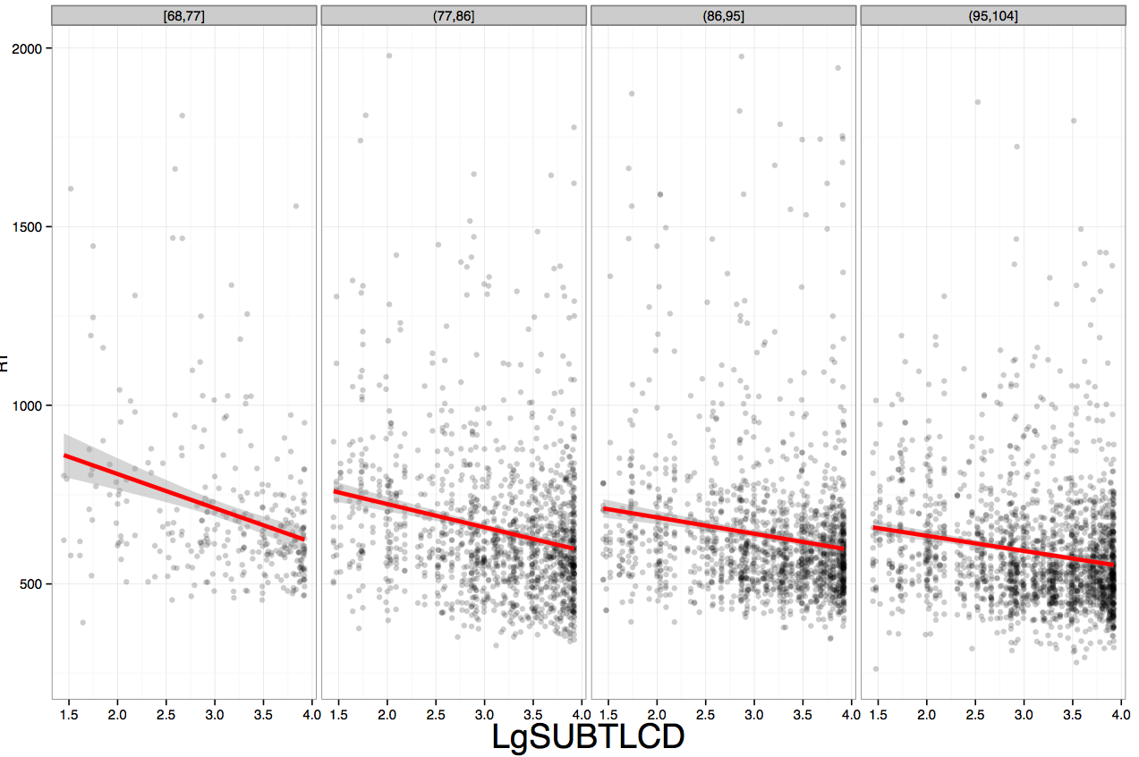
To me, there is a possible interaction such that the frequency effect (LgSUBTLCD) may be getting smaller for older readers but that modulation of frequency by age does not seem very strong.
OLS Regression — the full dataset
We can perform a full regression on the dataset to look for the effects of interest, effects of subject attributes, of word attributes and of the interactions between the first and the last. We are going to ignore the fact that, due to the dependencies of observations under subject and item, we do not really have as many degrees of freedom as we appear to have (several thousand observations).
We can run a regression taking all the data and ignoring the clustering of observations:
# Inspect the database

summary(nomissing.full)

# recommended that first make an object that summarizes the distribution

nomissing.full.dd <- datadist(nomissing.full)

# specify that will be working with the subjects.dd data distribution

options(datadist = "nomissing.full.dd")

# run the ols() function to perform the regression

nomissing.full.ols <- ols(logrt ~

(cAge + cTOWREW + cTOWRENW + cART)*
(cLength + cOLD + cIMG + cAOA + cLgSUBTLCD),

data = nomissing.full)

# enter the name of the model to get a summary

nomissing.full.ols
That will get you this:
# > nomissing.full.ols
#
# Linear Regression Model
#
# ols(formula = logrt ~ (cAge + cTOWREW + cTOWRENW + cART) * (cLength +
#                                                               cOLD + cIMG + cAOA + cLgSUBTLCD), data = nomissing.full)
#
# Model Likelihood     Discrimination
# Ratio Test           Indexes
# Obs     5257    LR chi2    677.56    R2       0.121
# sigma 0.1052    d.f.           29    R2 adj   0.116
# d.f.    5227    Pr(> chi2) 0.0000    g        0.043
#
# Residuals
#
# Min       1Q   Median       3Q      Max
# -0.37241 -0.06810 -0.01275  0.05202  0.55272
#
# Coef    S.E.   t       Pr(>|t|)
# Intercept              2.7789 0.0015 1914.52 <0.0001
# cAge                   0.0015 0.0001   13.95 <0.0001
# cTOWREW               -0.0018 0.0002   -8.42 <0.0001
# cTOWRENW               0.0009 0.0003    3.40 0.0007
# cART                  -0.0021 0.0002  -11.58 <0.0001
# cLength               -0.0101 0.0027   -3.68 0.0002
# cOLD                   0.0012 0.0071    0.18 0.8599
# cIMG                  -0.0066 0.0013   -5.00 <0.0001
# cAOA                   0.0022 0.0010    2.16 0.0310
# cLgSUBTLCD            -0.0365 0.0033  -10.98 <0.0001
# cAge * cLength         0.0003 0.0002    1.46 0.1453
# cAge * cOLD           -0.0006 0.0005   -1.13 0.2580
# cAge * cIMG            0.0000 0.0001   -0.03 0.9798
# cAge * cAOA           -0.0001 0.0001   -1.02 0.3099
# cAge * cLgSUBTLCD      0.0001 0.0002    0.42 0.6767
# cTOWREW * cLength      0.0002 0.0004    0.54 0.5915
# cTOWREW * cOLD         0.0002 0.0011    0.22 0.8265
# cTOWREW * cIMG         0.0000 0.0002    0.02 0.9859
# cTOWREW * cAOA         0.0002 0.0002    1.14 0.2531
# cTOWREW * cLgSUBTLCD   0.0002 0.0005    0.31 0.7600
# cTOWRENW * cLength    -0.0004 0.0005   -0.80 0.4213
# cTOWRENW * cOLD        0.0009 0.0012    0.72 0.4735
# cTOWRENW * cIMG        0.0003 0.0002    1.29 0.1975
# cTOWRENW * cAOA        0.0000 0.0002   -0.20 0.8377
# cTOWRENW * cLgSUBTLCD  0.0015 0.0006    2.62 0.0088
# cART * cLength        -0.0004 0.0003   -1.29 0.1967
# cART * cOLD            0.0002 0.0009    0.22 0.8263
# cART * cIMG           -0.0001 0.0002   -0.65 0.5133
# cART * cAOA            0.0000 0.0001    0.17 0.8670
# cART * cLgSUBTLCD     -0.0005 0.0004   -1.29 0.1964
which looks perfectly reasonable.
Notice:
— A regression model might be written as:

— I can break the function call down:
subjects.ols — the name of the model to be created
<- ols() — the model function call
TOWRE_wordacc — the dependent or outcome variable
~ — is predicted by
Age + TOWRE_nonwordacc + ART_HRminusFR — the predictors
, data = subjects — the specification of what dataframe will be used
— Notice also that when you run the model, you get nothing except the model command being repeated (and no error message if this is done right).
— To get the summary of the model, you need to enter the model name:
subjects.ols
— Notice when you look at the summary the following features:
Obs — the number of observations
d.f. — residual degrees of freedom
Sigma — the residual standard error i.e. the variability in model residuals — models that better fit the data would be associated with smaller spread of model errors (residuals)
Residuals — the listed residuals quartiles, an indication of the distribution of model errors — linear regression assumes that model errors are random, and that they are therefore distributed in a normal distribution
Model Likelihood Ratio Test — a measure of goodness of fit, with the 


In estimating the outcome (here, word reading skill), we are predicting the outcome given what we know about the predictors. Most of the time, the prediction will be imperfect, the predicted outcome will diverge from the observed outcome values. How closely do predicted values correspond to observed values? In other words, how far is the outcome independent of the predictor? Or, how much does the way in which values of the outcome vary coincide with the way in which values of the predictor vary? (I am paraphrasing Cohen et al., 2003, here.)
Let’s call the outcome Y and the predictor X. How much does the way in which the values of Y vary coincide with the way in which values of X vary? We are talking about variability, and that is typically measured in terms of the standard deviation SD or its square the variance 
Coef — a table presenting the model estimates for the effects of each predictor, while taking into account all other predictors
Notice:
— The estimated regression coefficients represent the rate of change in outcome units per unit change in the predictor variable.
— You could multiple the coefficient by a value for the predictor to get an estimate of the outcome for that value e.g. word reading skill is higher by 0.7382 times each unit increase in nonword reading score.
— The intercept (the regression constant or Y intercept) represents the estimated outcome when the predictors are equal to zero – you could say, the average outcome value assuming the predictors have no effect, here, a word reading score of 55.
For some problems, as here, it is convenient to center the predictor variables by subtracting a variable’s mean value from each of its values. This can help alleviate nonessential collinearity (see here) due to scaling, when working with curvilinear effects terms and interactions, especially (Cohen et al., 2003). If both the outcome and predictor variables have been centered then the intercept will also equal zero. If just the predictor variable is centered then the intercept will equal the mean value for the outcome variable. Where there is no meaningful zero for a predictor (e.g. with age) centering predictors can help the interpretation of results. The slopes of the effects of the predictors are unaffected by centering.
— In addition to the coefficients, we also have values for each estimate for:
S.E. — the standard error of the estimated coefficient of the effect of the predictor. Imagine that we sampled our population many times and estimated the effect each time: those estimates would constitute a sampling distribution for the effect estimate coefficient, and would be approximately normally distributed. The spread of those estimates is given by the SE of the coefficients, which can be calculated in terms of the portion of variance not explained by the model along with the SDs of Y and of X.
t — the t statistic associated with the Null Hypothesis Significance Test (NHST, but see Cohen, 1994) that the effect of the predictor is actually zero. We assume that there is no effect of the predictor. We have an estimate of the possible spread of coefficient estimate values, given repeated sampling from the population, and reruns of the regression – that is given by the SE of the coefficient. The t-test in general is given by:

therefore, for regression coefficients:

i.e. for a null hypothesis that the coefficient should be zero, we divide the estimate of the coefficient, B, by the standard error of possible coefficients, to get a t-statistic
Pr(>|t|) — we can then get the probability that a value of t this large or larger by reference to the distribution of t values for the degrees of freedom at hand.
But is this really the right thing to do?
As I discuss in my talk, it is not (slides to be uploaded). I have already alluded to the problem. The model makes sense on its face. And the effects estimates might be reasonable. The problem is that we are not really giving the randomness its due here. Did we really have 5250+ independent observations? How accurate are our estimates of the standard errors?
OLS Regression — the by-items mean RTs dataset
The field has long been aware of random variation in datasets like this, where we are examining the effect of e.g. word attributes on the responses of samples of participants in a repeated-measures design. The solution has not been to throw all the data into a regression. Rather, we have averaged responses to each item over participants. To put it another way, for each word, we have averaged over the responses recorded for the participants in our sample, to arrive at an average person response. The folk explanation for this procedure is that we are ‘washing out’ random variation to arrive at a mean response but if you consider discussions by e.g. Raaijmakers et al. (1999) it is not quite that simple (the whole problem turns on the ‘language as fixed effect’ issue, the paper is highly recommended). Let’s look at how this works for our data set.
Note I am going to be a bit lazy here and not centre the predictors before performing the analysis nor log transform RTs. You’re welcome to redo the analysis having made that preliminary step.
The first thing we need to do is create a database holding by-items mean RTs. We do this by calculating the average RT (over subjects) of responses to each item.
# define functions for use later:

# we want to examine performance averaging over subjects to get a mean RT for each item ie by items RTs

# first create a function to calculate mean RTs

meanRT <- function(df) {mean(df$RT)}

# then apply it to items in our original full dataset, outputting a dataset of by-items mean RTs

nomissing.full.byitems.RT.means <- ddply(nomissing.full, .(item_name), meanRT)

# inspect the results

summary(nomissing.full.byitems.RT.means)

# if you click on the dataframe name in the workspace window in RStudio you can see that we have created a set of 160
# (mean) RTs

# we want to rename the variable calculated for us from V1 to byitems.means

nomissing.full.byitems.RT.means <- rename(nomissing.full.byitems.RT.means, c(V1 = "byitems.means"))
The next thing we can do is add information about the items into this dataframe by merging it with our item norms dataframe, as follows:
# we can analyse what affects these by-items means RTs but must first merge this dataset with the item norms dataset:

byitems <- merge(nomissing.full.byitems.RT.means, item.words.norms, by = "item_name")

# inspect the results

summary(byitems)
We can then run another OLS regression, this time on just the by-items means RTs therefore without the subject attribute variables or, critically, the interactions, as follows:
# recommended that first make an object that summarizes the distribution

byitems.dd <- datadist(byitems)

# specify that will be working with the subjects.dd data distribution

options(datadist = "byitems.dd")

# run the ols() function to perform the regression

byitems.ols <- ols(byitems.means ~

Length + OLD + brookesIMG + AoA_Kup_lem + LgSUBTLCD,

data = byitems)

# enter the name of the model to get a summary

byitems.ols
That will get you this:
> byitems.ols

Linear Regression Model

ols(formula = byitems.means ~ Length + OLD + brookesIMG + AoA_Kup_lem +
LgSUBTLCD, data = byitems)

Model Likelihood     Discrimination
Ratio Test           Indexes
Obs       160    LR chi2    126.84    R2       0.547
sigma 39.8543    d.f.            5    R2 adj   0.533
d.f.      154    Pr(> chi2) 0.0000    g       47.664

Residuals

Min       1Q   Median       3Q      Max
-96.8953 -26.1113  -0.3104  20.8134 167.8680

Coef     S.E.    t     Pr(>|t|)
Intercept   912.2377 49.6487 18.37 <0.0001
Length      -19.2256  5.8640 -3.28 0.0013
OLD           6.5787 15.2532  0.43 0.6669
brookesIMG  -12.6055  2.8667 -4.40 <0.0001
AoA_Kup_lem   4.0169  2.2254  1.81 0.0730
LgSUBTLCD   -58.1738  7.1677 -8.12 <0.0001
Notice:
— the proportion of variance explained by the model is considerably larger than that explained by the model for the full dataset
— the residual standard error is also larger
— obviously the degrees of freedom are reduced
— the pattern of effects seems broadly similar i.e. what effects are significant and what are not
How could we take into account both random variation due to items (as in our by-items analysis) and random variation due to subjects?
As I discuss in my talk (slides to be uploaded here), discussions by Clark (1973), Raaijmakers et al. (1999) are enlightening. We are heading towards the mixed-effects approach argued by Baayen (2008; Baayen et al., 2008) and many others to do the job. We might consider one last option, to perform a by-items analysis not on by-items mean RT but on the RTs of each participant considered as an individual (seeLorch & Myers, 1990). We might then analyse the coefficients resulting from that per-subjects analysis: see Balota et al. (2004), for one example of this approach; see Snijders & Boskers (1999), also Baayen et al. (2008), for a discussion of the problems with it.
We can first define a function to perform a regression analysis for each subject:
model <- function(df){lm(logrt ~

Length + OLD + brookesIMG + AoA_Kup_lem +
LgSUBTLCD,

data = df)}
Notice:
— I am switching to the lm() function to run regression analyses — the effect is the same but the function will be a bit simpler to handle.
Then use the function to model each person individually, creating a dataframe with results of each model:
nomissing.full.models <- dlply(nomissing.full, .(subjectID), model)

rsq <- function(x) summary(x)$r.squared
nomissing.full.models.coefs <- ldply(nomissing.full.models, function(x) c(coef(x),rsquare = rsq(x)))

head(nomissing.full.models.coefs,n=3)
length(nomissing.full.models.coefs$subjectID)
summary(nomissing.full.models.coefs)

# then merge the models coefs and subject scores dbases by subject

nomissing.full.models.coefs.subjects <- merge(nomissing.full.models.coefs, subjects, by="subjectID")

# inspect

summary(nomissing.full.models.coefs.subjects)
We can use these data to analyse whether coefficients of effects of word attributes estimated separately for each subject are, themselves, estimatble given data about subject attributes.
# we can now analyse whether the coefficients are predicted by subject variables

# rename the dataframe for simplicity:

subjects.coefs <- nomissing.full.models.coefs.subjects

# recommended that first make an object that summarizes the distribution

subjects.coefs.dd <- datadist(subjects.coefs)

# specify that will be working with the subjects.dd data distribution

options(datadist = "subjects.coefs.dd")

# run the ols() function to perform the regression

subjects.coefs.ols <- ols(LgSUBTLCD ~

Age + TOWRE_wordacc + TOWRE_nonwordacc + ART_HRminusFR,

data = subjects.coefs)

# enter the name of the model to get a summary

subjects.coefs.ols
Running that code will get you this:
> subjects.coefs.ols

Linear Regression Model

ols(formula = LgSUBTLCD ~ Age + TOWRE_wordacc + TOWRE_nonwordacc +
ART_HRminusFR, data = subjects.coefs)

Model Likelihood     Discrimination
Ratio Test           Indexes
Obs       34    LR chi2     19.94    R2       0.444
sigma 0.0176    d.f.            4    R2 adj   0.367
d.f.      29    Pr(> chi2) 0.0005    g        0.015

Residuals

Min        1Q    Median        3Q       Max
-0.029786 -0.014093  0.002851  0.012819  0.032995

Coef    S.E.   t     Pr(>|t|)
Intercept        -0.1264 0.0328 -3.86 0.0006
Age               0.0001 0.0002  0.55 0.5856
TOWRE_wordacc     0.0001 0.0005  0.11 0.9101
TOWRE_nonwordacc  0.0017 0.0005  3.26 0.0029
ART_HRminusFR    -0.0006 0.0004 -1.57 0.1268
Notice that the effect of frequency does appear to be predicted by the effect of subject nonword reading performance — in line with the frequency x nonword interaction seen in the analysis of the full dataset, above.
What have we learnt?
datadist()
ols()
ddply()
ggplot() — see previous posts on data visualization
Reading
Baayen, R. H. (2008). Analyzing linguistic data. Cambridge University Press.
Baayen, R. H., Davidson, D. J., & Bates, D. M. (2008). Mixed-effects modeling with crossed random effects for subjects and items. Journal of memory and language, 59(4), 390-412.
Balota, D. A., Cortese, M. J., Sergent-Marshall, S. D., Spieler, D. H., & Yap, M. (2004). Visual word recognition of single-syllable words. Journal of Experimental Psychology: General, 133(2), 283.
Cohen, J., Cohen, P., West, S. G., & Aiken, L. S. (2003). Applied multiple regression/correlation analysis for the behavioural sciences (3rd. edition). Mahwah, NJ: Lawrence Erlbaum Associates.
Harrell Jr, F. J. (2001). Regression modelling strategies: With applications to linear models, logistic regression, survival analysis. New York, NY: Springer.
Lorch, R. F., & Myers, J. L. (1990). Regression analyses of repeated measures data in cognitive research. Journal of Experimental Psychology: Learning, Memory, and Cognition, 16(1), 149.
Raaijmakers, J. G., Schrijnemakers, J., & Gremmen, F. (1999). How to deal with “the language-as-fixed-effect fallacy”: Common misconceptions and alternative solutions. Journal of Memory and Language, 41(3), 416-426.
Snijders, T. A. B., & Bosker, R. J. (1999). Multilevel analysis: An introduction to basic and advanced multilevel modelingSage Publications. Thousand Oaks, CA.
