This post will be one of four in which we go through how to model a multilevel dataset using linear mixed-effects modeling. To begin, we need to collate the data we have gathered in a simple reading experiment but one involving a repeated-measures design warranting a mixed-effects approach.

Data handling

This post is an updated version of an earlier post. The .R code I will use to perform the operations discussed in this post can be downloaded from here.

I am going to assume that you know how to install R and RStudio, if not, see earlier posts or this recent summary where you are shown how to:

— install R (the statistical programming environment) and RStudio (the interactive editor for working with R)

— start a script to run R functions and get things done

— install R packages to gain access to the capabilities furnished by user-contributed libraries of functions

— can write and run R code to e.g. produce basic plots or get summary statistics

–download data files of the sort we will be using (.csv) and read them into R workspace as dataframes

You should also know how to get help in R, as summarized here.

What we will do in this post is focus on getting your data together in preparation for running mixed-effects modelling

The data we will use in our example were collected for a student research project. We were interested in whether or how lexical decision responses were influenced by:

1. the participant attributes;

2. the item attributes;

3. interactions between participant and item attributes.

We tested 39 adults, males and females, most either in their 20s or in middle age.

Every adult was tested on word and nonword reading skills (TOWRE, Torgesen et al., 1999) and print exposure (ART, Masterson & Hayes, 2007). We collated the subject scores database and it can be downloaded here.

Critically, every adult also was tested in a computer based lexical decision task (run using DMDX, Forster & Forster, 2003) in which they saw 320 letter strings on a screen, one at a time, and were asked to indicate by a button press (using a gamepad) whether they thought each item was a word they knew or a nonword they did not. In addition to the 320 critical trials, participants were also given 20 practice trials which we shall ignore in the analysis. Information on the item names (the word or non-word) linking them to item type (word or non-word) and item number (DMDX trial number) can be downloaded here, we will need it for later merge operations.

The words and nonwords were selected to be matched on length (measured in letters), orthographic neighbourhood size (often called N, Coltheart et al., 1977) and bigram frequency (mean, sum and frequency specific numbers). This matching was designed to force participants to access their mental lexicon to perform the task, instead of making responses based on ‘low-level’ perceptual information like item length. We collated data on item (word and nonword attributes) and they can be downloaded here, see relevant previous posts here and here.

However, what we really cared about, in designing the experiment, was whether the time that participants took to respond to stimuli (reaction time, RT, or response latency) – the interval from stimulus onset to response onset – varied in relation to: participant attributes like reading skill; item attributes like length; and the interactions between those two sets of predictors. In addition to the length etc. of the items, we also cared if lexical access was influenced by word attributes. Focusing on just words, we wanted to know if RTs were affected by word frequency, age of acquisition (AoA), and imageability. We collated information about such attributes and combined them with data on item attributes like length to a single database that can be downloaded here, see relevant post here.

All these data about item attributes were drawn either from the English Lexicon Project (Balota et al., 2007) or from datasets very helpfully provided by other psycholinguists (Cortese & Fuggett, 2004; Cortese & Khanna, 200; Kuperman et al., in press) see notes here and here.

When we ran the lexical decision study, DMDX produced an .azk output file holding keypress RTs along with information about trial order (when did a word appear in a block of stimulus trials) and participant identity code (subjectID).

Getting data recorded in an experiment into a usable state can be a quite exasperating process. Things that one encounters include: inconsistent subjectID naming between behavioural and participant attribute data collection; item or trial coding errors; mismatches because one used the word false in excel. For some reason, the process of data collation is often called data munging.

The behavioural data file is in ‘long format’: all participants tested are shown, one participant on top of the other, in a long column where each row corresponds to a single trial observation, i.e. each row corresponds to a response made by a participant to a word. It can be downloaded here.

If you open it in excel, it looks like this:

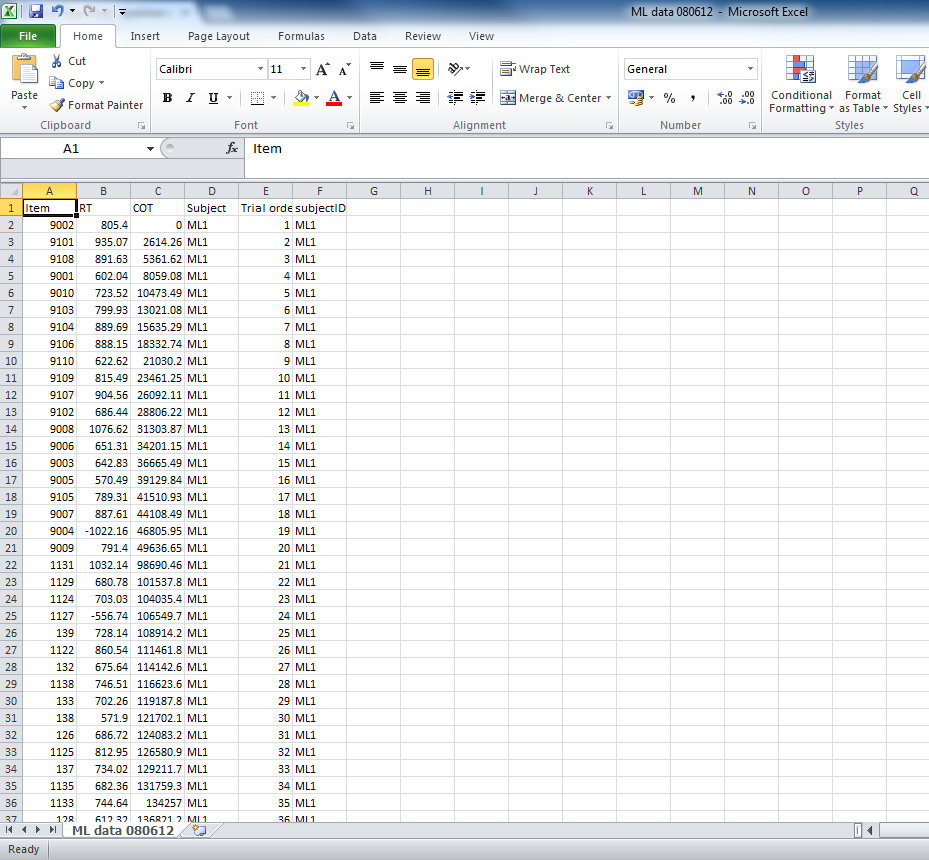
Notice:

— If you were to open the file in excel, you would see that there are 13941 rows, including the column headers or variable names.

— 13940 data rows =  340*41

– Recall I said there were 320 critical trials and 39 participants. On the latter score, I misspoke: we lost two because of inconsistent subjectID entry. If you don’t know who they are (or, at least, if you cannot map subjectIDs in a participant attributes to subjectIDs in a behavioural database), you cannot analyze them.

Load the data into the workspace

I am going to assume you have successfully downloaded the datafiles and have them in a folder that you are able to use as your working directory.

You can run the following code to set the working directory to the folder where the datafiles are and then load the files into the R session workspace as dataframes.

# set the working directory

setwd("[enter path to folder holding data files here]")

# # read in the item norms data
#
# item.norms <- read.csv(file="item norms 270312 050513.csv", head=TRUE,sep=",", na.strings = "-999")
# word.norms <- read.csv(file="word norms 140812.csv", head=TRUE,sep=",", na.strings = "-999")

item.coding <- read.csv(file="item coding info 270312.csv", head=TRUE,sep=",", na.strings = "-999")

# read in the merged new dataframe

item.words.norms <- read.csv(file="item.words.norms 050513.csv", head=TRUE,sep=",", na.strings = "NA")

# read in the subjects scores data file

subjects <- read.csv("ML scores 080612 220413.csv", header=T, na.strings = "-999")

# read in the behavioural data file

behaviour <- read.csv("ML data 080612.csv", header=T, na.strings = "-999")

Notice:

— I commented out the read.csv() function calls for item.norms and word.norms. We will not need that stuff for this post.

— We do now need the item.coding dataframe, however, for reasons I will explain next.

Put the databases together

We next need to put the dataframes together through the use of the merge() function.

What this means is that we will end up with a dataframe that:

1. has as many rows (some thousands) as valid observations

2. each observation will be associated with data about the subject and about the word.

Notice:

— The merge() function  (see the help page) allows you to put two dataframes together. I believe other functions allow merger of multiple dataframes.

— By default, the dataframes are merged on the columns with names they both have, so here we plan to merge: the normative item.words.norms dataframe with the item.coding dataframe by the common variable item_name; we then merge that norms.coding dataframe with the behaviour dataframe by the common variable item_number; we then merge that RTs.norms dataframe with the subject scores dataframe by the common variable subjectID.

— You see why we needed the coding data: the behavioural database lists RT observations by (DMDX trial item) number; the normative database lists item attribute observations by item name (e.g. a word name like “axe”); I cannot put the normative and the behavioural databases without a common variable, that common variable has to be item_name so I created the coding database, deriving the information from the DMDX script, to hold both the item_name and item_number columns. Creating the coding database was not too costly but the fact that I needed to do so illustrates the benefits of thinking ahead, if I had thought ahead, I would have had both item_name and item_number columns in the normative database when I built it.

— As noted previously, if the dataframes being merged do not have observations that cannot be mapped together because there is a mismatch on the row index e.g. item name or whatever other common variable is being used they get ‘lost’ in the process of merging. This is nicely illustrated by what happens when you merge the behaviour dataframe – which holds observations on both responses to words and to nonwords – with the item.words.norms dataframe, which holds just data about the attributes of words. As there are no nonword  items in the latter, when you merge item.words.norms and behaviour, creating a new joint dataframe, the latter has nothing about nonwords. This suits my purposes, because I wish to ignore nonwords (and practice items, for that matter, also absent from the norms database) but you should pay careful attention to what should happen and what does happen when you merge dataframes.

— I also check my expectations about the results of operations like merge() against the results of those operations. I almost never get a match first time between expectations and results. Here, it is no different, as I will explain.

Let’s run the code to merge our constituent databases.

# to put files together ie to merge files we use the merge() function
# we want to put the data files together so that we can analyze RTs by subject characteristics or item norms or conditions (coding)

# so that we can associate item normative with coding data, we need to merge files by a common index, item_name

norms.coding <- merge(item.words.norms, item.coding, by="item_name")

# inspect the result

head(norms.coding, n = 2)

# note the common index item_name does not get repeated but R will recognize the duplication of item_type and assign .x or .y
# to distinguish the two duplicates.

# delete the redundant column

norms.coding <- norms.coding[, -2] # using data file indexing, [,] - to remove, remove 2 the second column

head(norms.coding,n=2)

# rename the .y column to keep it tidy

norms.coding <- rename(norms.coding, c(item_type.y = "item_type"))

# inspect the results:

head(norms.coding,n=2)

summary(norms.coding)

# put the data files together with data on subjects and on behaviour:

# first, rename "Item" variable in lexical.RTs as "item_number" to allow merge

behaviour <- rename(behaviour, c(Item = "item_number"))

# run merge to merge behaviour and norms

RTs.norms <- merge(norms.coding, behaviour, by="item_number")

# run merge to merge RTs.norms and subject scores

RTs.norms.subjects <- merge(RTs.norms, subjects, by="subjectID")

Notice:

— In merging the normative and coding dataframes, I had to deal with the fact that both held two common columns, the one I used for merging, item_name, and another, item_type. The former is used for merging and goes into the dataframe that is the product of the merger as a single column. The item_type column was not used for merging and consequently is duplicated: R deals with duplicates by renaming them to keep them distinct, here adding .x or .y.  This is a bit of a pain so I dealt with the duplication by deleting one copy and renaming the other.

If we inspect the results of the merger:

# inspect the results:

head(RTs.norms.subjects,n=2)
summary(RTs.norms.subjects)
length(RTs.norms.subjects$RT)

We see:

Notice:

— We have just observations of words: see the item_type summary.

— Participants, at least the first few, are listed under subjectID with 160 observations each, as they should be. Variables appear to be correctly listed by data type, numeric, factor etc.

— I note that there are some missing values, NAs, among the IMG and AOA observations.

— I also note that the Subject variable indicates at least one participant, A18, has 320 not 160 observations.

Checking: Does the merger output dataframe match my expectations?

As noted in the foregoing study summary, we have participant attribute data on 39 participants and, presumably, lexical decision behavioural data on those same participants. I would expect the final merger output dataframe, therefore, to have: 39*160 = 6240 rows.

It does not.

We need to work out what the true state of each component dataframe is to make sense of what we get as the output of the merge() calls.

The first thing I am going to do is to check if the merger between subjects and behaviour dataframes lost a few observations because there was a mismatch on subjectID for one or more participants. The way you can do this (there are smarter ways) is ask R what the levels of the subjectID factor are for each dataframe then check the matching by eye.

# how many rows should we have?

levels(subjects$subjectID)
levels(behaviour$subjectID)
levels(RTs.norms.subjects$subjectID)

Which shows you this:

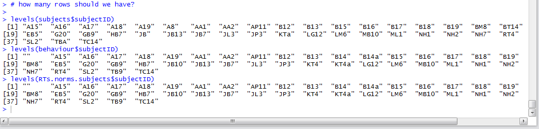
I can tell that there are some subjectIDs in the subjects dataframe that are not in the behaviour dataframe, and vice versa. Well, I told you that there were problems in the consistency of subjectID naming. The output dataframe RTs.norms.subjects will only have observations for those rows indexed with a subjectID in common between both behaviour and subjects dataframes. (I think the smarter way to do the check would be to do a logic test, using ifelse(), with a dataframe output telling you where subjectID is or is not matched.)

Notice:

— The behaviour dataframe includes 41 not 39 participants’ data, including one with a blank “” subjectID.

— The levels listed for subjectID for the output dataframe RTs.norms.subjects actually gives you all levels listed for both factors, irrespective of whether there are other data associated with each level. This is an artifact of the way in which R (otherwise efficiently) stores factors as indices, with instances.

— We need, therefore, to count how many observations we have for each participant in the output dataframe. I will do this by creating a function to count how many times subjectID is listed.

The following code using the function definition syntax in R as well as the ddply() function made available by installing the plyr package and then loading its library. The plyr package, by Hadley Wickham, is incredibly useful, and I will come back to it. If you copy the following code into the script window and then run it, we will see what it does, promising to return in a later post to explain what is going on and how it happens.

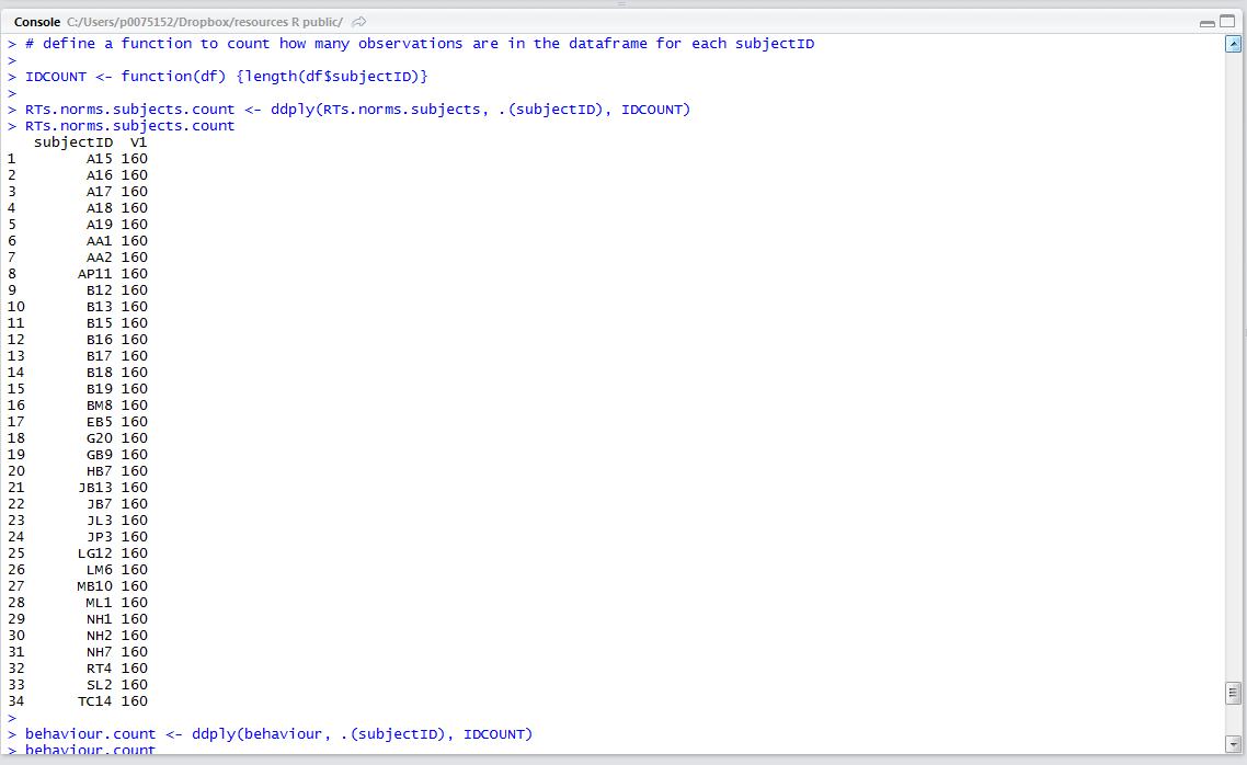
# define a function to count how many observations are in the dataframe for each subjectID

IDCOUNT <- function(df) {length(df$subjectID)}

RTs.norms.subjects.count <- ddply(RTs.norms.subjects, .(subjectID), IDCOUNT)
RTs.norms.subjects.count

behaviour.count <- ddply(behaviour, .(subjectID), IDCOUNT)
behaviour.count

Which gives you this:

What we have done is:

1. Created a function to count how many times each different subjectID value e.g. A15 occurs in the subjectID column. You should realize, here, that each subjectID will be listed in the subjectID column for every single row held, i.e. every observation recorded, in the dataframe for the participant.

2. Used the function to generate a set of numbers – for each participant, how many observations are there? – then used the ddply() function call to create a dataframe listing each subjectID with, for each one, the number of associated observations.

3. Inspecting the latter dataframe tells us that we have 35 participants with 160 observations for each one.

Neat, even if I do say so myself, but it is all thanks to the R megastar Hadley Wickham, see here for more information on plyr.

I think I now understand what happened:

1. We had a match on observations in the subject attributes data and the behavioural data for only 34 participants.

2. The output output dataframe RTs.norms.subjects therefore holds only 34 * 160 = 5440 observations.

Output the merged dataframe as a .csv file

Having done all that work (not really, I did in a few lines of code and milliseconds what hours of hand copy/pasting required), I don’t want to have to do it all again, therefore, I can create a .csv file using the write.csv() function.

# we can write the dataframe output by our merging to a csv file to save having to do this work again later

write.csv(RTs.norms.subjects, file = "RTs.norms.subjects 061113.csv", row.names = FALSE)

What have we learnt?

You could do this by hand. That would involve working in excel, and copying, for each person’s trials, their scores on the reading skill tests etc., and for each word, that word’s values on length etc. I have done that. It is both time-consuming and prone to human error. Plus, it is very inflexible because who wants to do a thing like that more than once? I learnt about keeping different datasets separate until needed – what you could call a modular approach – in the great book on advanced regression by Andrew Gelman and Jennifer Hill (Gelman & Hill, 2007).

I think that keeping data sets the right size – i.e. subject attributes data in a subjects data base, item attributes data in a normative data base etc. – is helpful, both more manageable (easier to read things, if required, in excel), less error prone, and logically transparent (therefore, in theory, more intuitive). However, the cost of using merge(), as I have shown, is that you are required to know exactly what you have, and what you should get. You should have that understanding anyway, and I would contend that it is easier to avoid feeling the obligation when working with excel or SPSS, but that that avoidance is costly in other words (reputational risk). Thus, work and check your workings. Just because they taught you that in school does not stop it from continuing relevance.

Key vocabulary

merge()

levels()

function{}

ddply()

length()

summary()

write.csv()

Reading

Balota, D. A., Yap, M.J., Cortese, M.J., Hutchison, K.A., Kessler, B., Loftus, B., . . . Treiman, R. (2007). The English lexicon project. Behavior Research Methods, 39, 445-459.
Coltheart, M., Davelaar, E., Jonasson, J. T., & Besner, D. (1977). Access to the internal lexicon. In S. Dornic (Ed.), Attention and Performance VI (pp. 535-555). Hillsdale,NJ: LEA.
Cortese, M.J., & Fugett, A. (2004). Imageability Ratings for 3,000 Monosyllabic Words. Behavior Methods and Research, Instrumentation, & Computers, 36, 384-387.
Cortese, M.J., & Khanna, M.M. (2008). Age of Acquisition Ratings for 3,000 Monosyllabic Words. Behavior Research Methods, 40, 791-794.
Gelman, A., & Hill, J. (2007). Data analysis using regression and multilevel/hierarchical models. New York,NY: Cambridge University Press.
Kuperman, V., Stadthagen-Gonzales, H., & Brysbaert, M. (in press). Age-of-acquisition ratings for 30 thousand English words. Behavior Research Methods.
Masterson, J., & Hayes, M. (2007). Development and data for UK versions of an author and title recognition test for adults. Journal of Research in Reading, 30, 212-219.
Torgesen, J. K., Wagner, R. K., & Rashotte, C. A. (1999). TOWRE Test of word reading efficiency. Austin,TX: Pro-ed.