This post assumes that you have installed R and R-studio, see here and here if not.

Getting started with data analysis can require a shift in mind-set.

Home base for most people is a spreadsheet

Most people find it difficult to start using R because they are most comfortable with something that resembles a physical version of their data, an SPSS or excel spreadsheet.

I assume you have seen a spreadsheet of data looking like this:

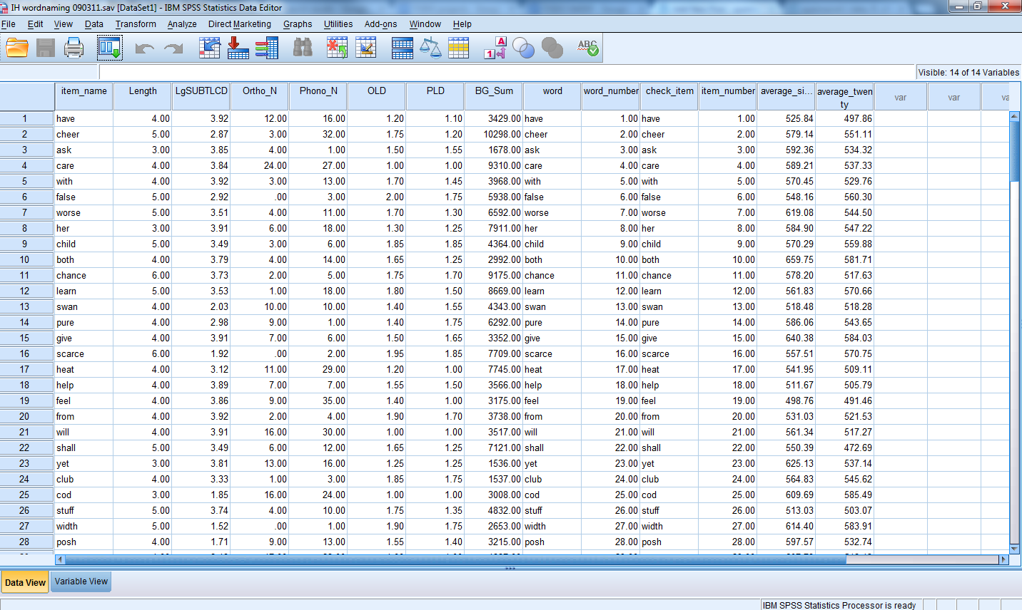
Notice:

— You can see a table of columns and rows. The columns have names like Length and the rows have numbers (on the far left).

— At the intersection of each column and row there’s a cell.

— There are scroll bars on the right, for vertical scrolling, and at the bottom, for horizontal scrolling.

This is SPSS but excel will show you something similar if you open an .xlsx spreadsheet. You can move around it and interact with it like any other thing in the world. Except, of course, it would be a mistake to think of a spreadsheet like that because what counts is the information, and the capacity to address, manipulate and analyse it.

R basics – the data objects

I have referred previously to the R workspace, objects, dataframes and variables, as here and here, where we read in a data file on participant scores in reading and other tests for a reading experiment, and drew some plots like histograms and scatterplots.

Before we go on, we need to firm up our understanding of how data are represented and analysed in R.

R is a language and you learn that language to create and manipulate objects (see the R intro). During data analysis, objects are created and stored by name.

[Think about the cultural difference here, compared to SPSS and excel: sure, in those applications, you call your data files and your variables by name but, because you can scroll around the data files i.e. spreadsheets, the variable names you use can be useless (meaningless, imprecise, poorly remembered etc.) but that need not stop you because they are things with locations in a field (the spreadsheet) and you can find a datum in a .sav or .xlsx file simply by looking, just as you can see a poppy in a wheat field even when ignorant of its name.]

The collection of objects currently stored is the workspace. You might keep data files in a folder on your computer, and you will direct R to that folder as a working directory, using the setwd() function. But you will load data files (e.g. a .csv file) using the read.csv() function — or some other version of read() — stored in the working directory to make them available to R as objects in the workspace. (Got it? See this Quick-R post for help.)

If you’re using R you’re dealing with data.

Data structures and data modes

R deals with data in a variety of types or structures: scalars, vectors, arrays, matrices, dataframes and lists. This diversity is one reason R is so flexible, and thus, powerful.

A dataframe is equivalent to the spreadsheet in SPSS or excel: a rectangular collection of data arranged in columns (variables or attributes) and rows (observations or cases)

There are different structures but also different data types or modes. R can deal with: numeric, character, logical and other types of data.

[Search “mode” in flickr Creative Commons and this what you get, US National Archives: mounted horsemen, awaiting the start of a parade, Cotton Wood Falls, Kansas, 1974]

The entities R operates on are objects. Objects have properties (or attributes) like their mode or length.

Vectors

You could have a chain or sequence or one-dimensional array of numbers or logical values or words (character strings): a vector of numeric values; logical values or character strings.

Vectors must have their values all of the same mode. A vector can be empty and still have a mode.

You can create a vector using the c() function: I think c means concatenate i.e. to chain things together.

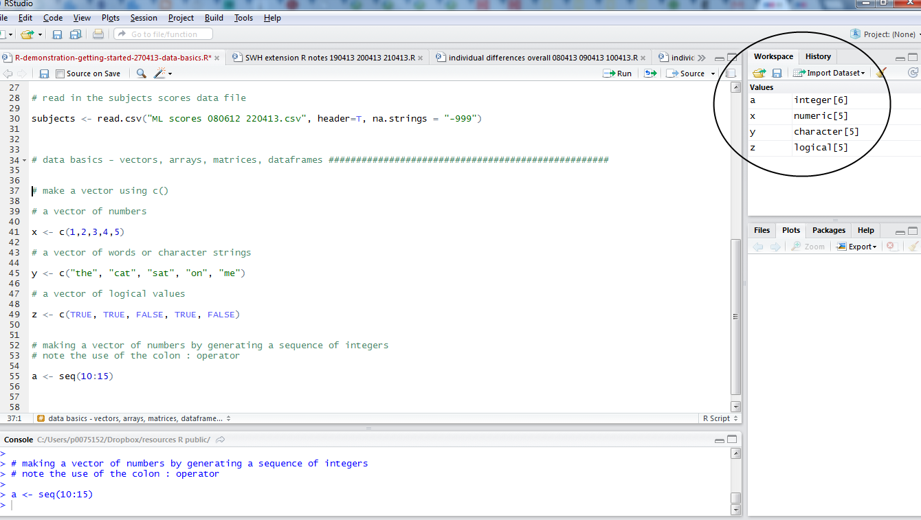
# data basics - vectors, arrays, matrices, dataframes ###################################################

# make a vector using c()

# a vector of numbers

x <- c(1,2,3,4,5)

# a vector of words or character strings

y <- c("the", "cat", "sat", "on", "me")

# a vector of logical values

z <- c(TRUE, TRUE, FALSE, TRUE, FALSE)

# making a vector of numbers by generating a sequence of integers
# note the use of the colon : operator

a <- seq(10:15)

If you run this code in R, you can see each vector being listed in the workspace as an object – vectors of varying mode – after the function call.

The data in a vector must be of only one type or  mode.

Scalars are vectors of one element, and are used to hold constants.

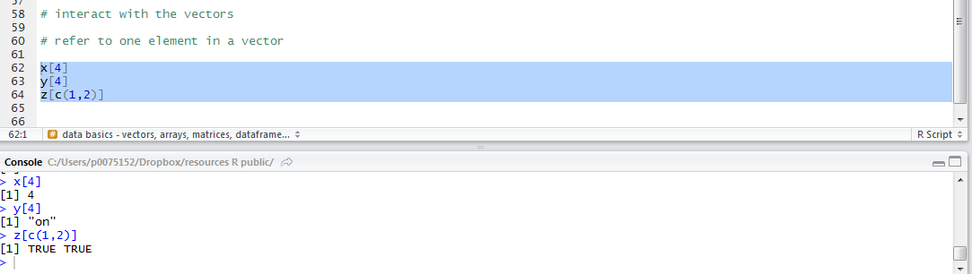
You can interact with the vectors – they are objects.

You can refer to an element by place or position, specifying place by number within square brackets. For example, for the vectors produced in the foregoing, the fourth place element is, or the first and the second elements are:

x[4]
y[4]
z[c(1,2)]

Run those lines of code and you’ll see:

Matrices

Arrays

Dataframes

— to follow

There are also objects called lists with the mode list. These are ordered sequences of objects which can each be of any modes (including list – you could have a list of lists).

Further reading

Read the R-in-Action book or the Quick-R blog, or indeed the R introduction, for further help but, honestly, the information you need is all over the internet.