Install R

Revise how to install R, as previously discussed here and here.

Installation

How do you download and install R? Google “CRAN” and click on the download link, then follow the instructions (e.g. at “install R for the first time”).

Anthony Damico has produced some great video tutorials on using R, here is his how-to guide:

http://www.screenr.com/kzT8

And moonheadsing at Learning Omics has got a blog post with a series of screen-shots showing you how to install R with pictures.

Install R-studio

Having installed R, the next thing we will want to do is install R-studio, a popular and useful interface for writing scripts and using R.

If you google “R-studio” you will get to this window:

Click on the “Download now” button and you will see this window:

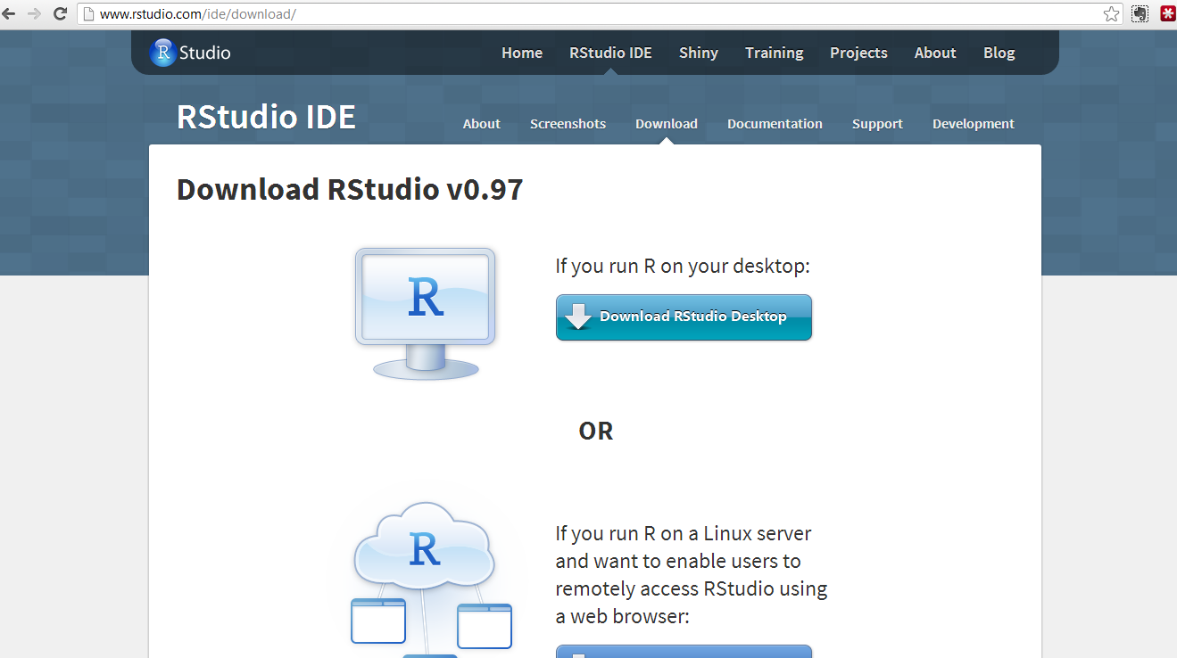
Click on the “Download RStudio desktop” and you will see this window:

You can just click on the link to the installer recommended for your computer.

What happens next depends on whether you have administrative/root privileges on your computer.

I believe you can install R-studio without such rights using the zip/tarball dowload.

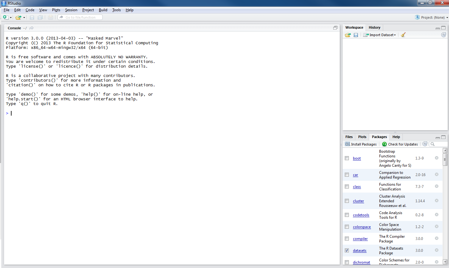
Having installed R and R-studio,  in Windows you will see these applications now listed as newly installed programs at the start menu. Depending on what you said in the installation process, you might also have icons on your desktop.

Click on the R-studio icon – it will pick up the R installation for you.

Now we are ready to get things done in R.

Start a new script in R-studio, install packages, draw a plot

Here, we are going to 1. start a new script, 2. install then load a library of functions (ggplot2) and 3. use it to draw a plot.

Depending on what you did at installation, you can expect to find shortcut links to R (a blue R) and to R-Studio (a shiny blue circle with an R) in the Windows start menu, or as icons on the desktop.

To get started, in Windows, double click (left mouse button) on the R-Studio icon.

Maybe you’re now looking at this:

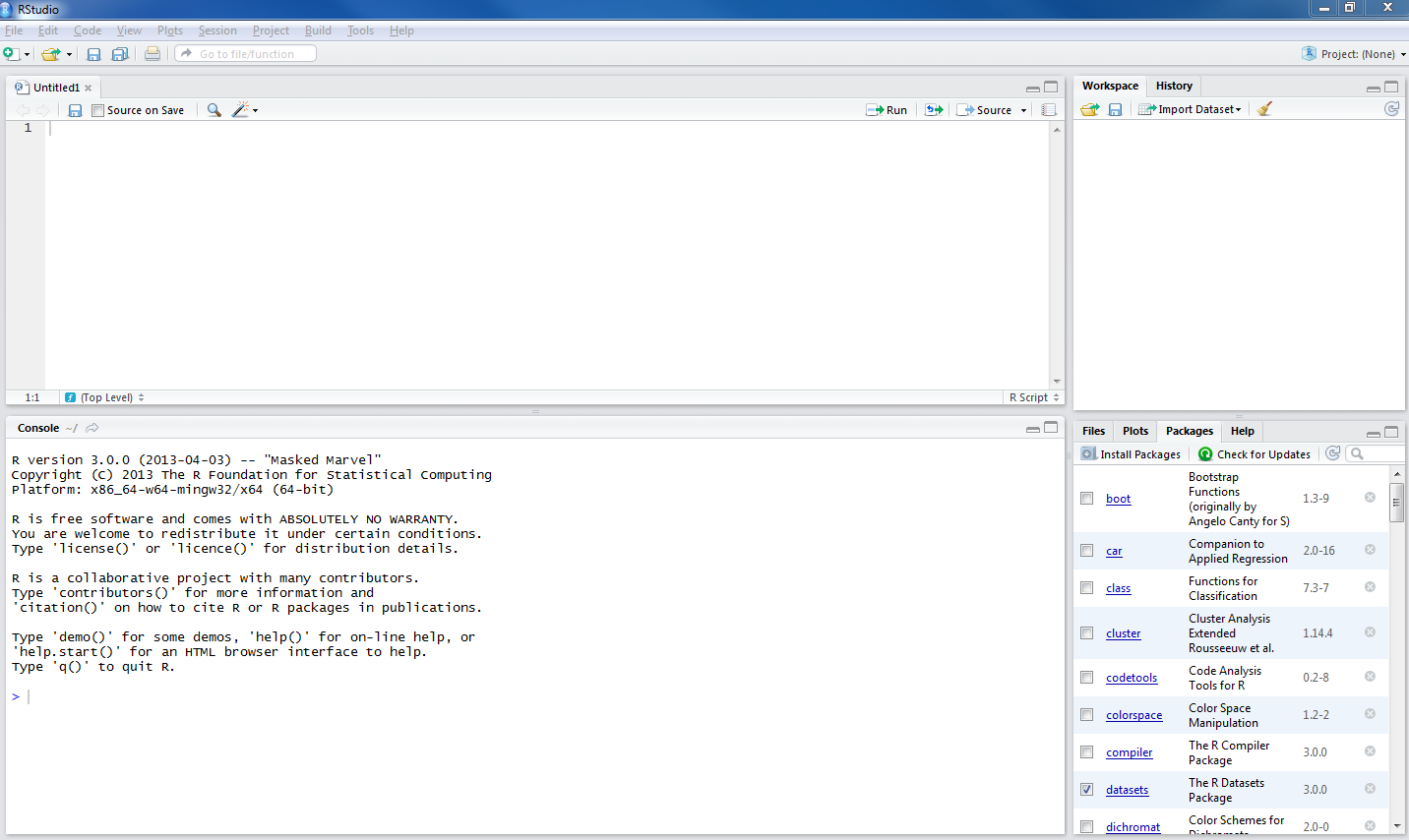
1. Start a new script

What you will need to do next is go to the file menu [top left of R-Studio window] and create a new R script:

–move the cursor to file – then – new – then – R script and then click on the left mouse button

or

— just press the buttons ctrl-shift-N at the same time — the second move is a keyboard shortcut for the first, I prefer keyboard short cuts to mouse moves

— to get this:

What’s next?

This circled bit you see in the picture below:

is the console.

It is what you would see if you open R directly, not using R-Studio.

You can type and execute commands in it but mostly you will see unfolding here what happens when you write and execute commands in the script window, circled below:

— The console reflects your actions in the script window.

If you look on the top right of the R-Studio window, you can see two tabs, Workspace and History: these windows (they can be resized by dragging their edges) also reflect what you do:

1. Workspace will show you the functions, data files and other objects (e.g. plots, models) that you are creating in your R session.

[Workspace — See the R introduction, and see the  this helpful post by Quick-R — when you work with R, your commands result in the creation of objects e.g. variables or functions, and during an R session these objects are created and stored by name — the collection of objects currently stored is the workspace.]

2. History shows you the commands you execute as you execute them.

— I look at the Workspace a lot when using R-Studio, and no longer look at (but did once use) History much.

My script is my history.

2. Install then load a library of functions (ggplot2)

We can start by adding some capacity to the version of R we have installed. We install packages of functions that we will be using e.g. packages for drawing plots (ggplot2) or for modelling data (lme4).

[Packages – see the introduction and this helpful page in Quick-R — all R functions and (built-in) datasets are stored in packages, only when a package is loaded are its contents available]

Copy then paste the following command into the script window in R-studio:

install.packages("ggplot2", "reshape2", "plyr", "languageR",
"lme4", "psych")

Highlight the command in the script window …

— to highlight the command, hold down the left mouse button, drag the cursor from the start to the finish of the command

— then either press the run button …

[see the run button on the top right of the script window]

… or press the buttons CTRL-enter together, and watch the console show you R installing the packages you have requested.

Those packages will always be available to you, every time you open R-Studio, provided you load them at the start of your session.

[I am sure there is a way to ensure they are always loaded at the start of the session and will update this when I find that out.]

There is a 2-minute version of the foregoing laborious step-by-step, by ajdamico, here. N.B. the video is for installing and loading packages using the plain R console but applies equally to R-Studio.

Having installed the packages, in the same session or in the next session, the first thing you need to do is load the packages for use by using the library() function:

library(languageR)
library(lme4)
library(ggplot2)
library(rms)
library(plyr)
library(reshape2)
library(psych)

— copy/paste or type these commands into the script, highlight and run them: you will see the console fill up with information about how the packages are being loaded:

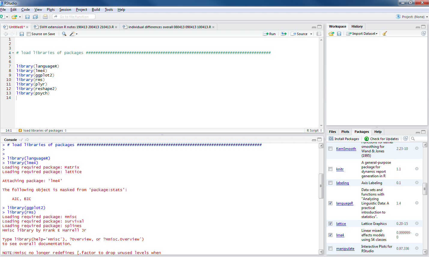
Notice that the packages window on the bottom right of R-Studio now shows the list of packages have been ticked:

Let’s do something interesting now.

3. Use ggplot function to draw a plot

[In the following, I will use a simple example from the ggplot2 documentation on geom_point.]

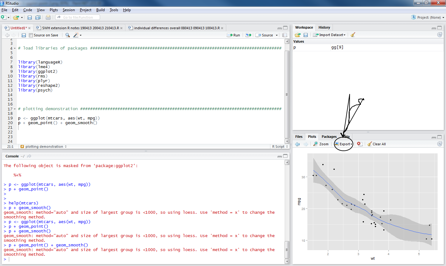
Copy the following two lines of code into the script window:

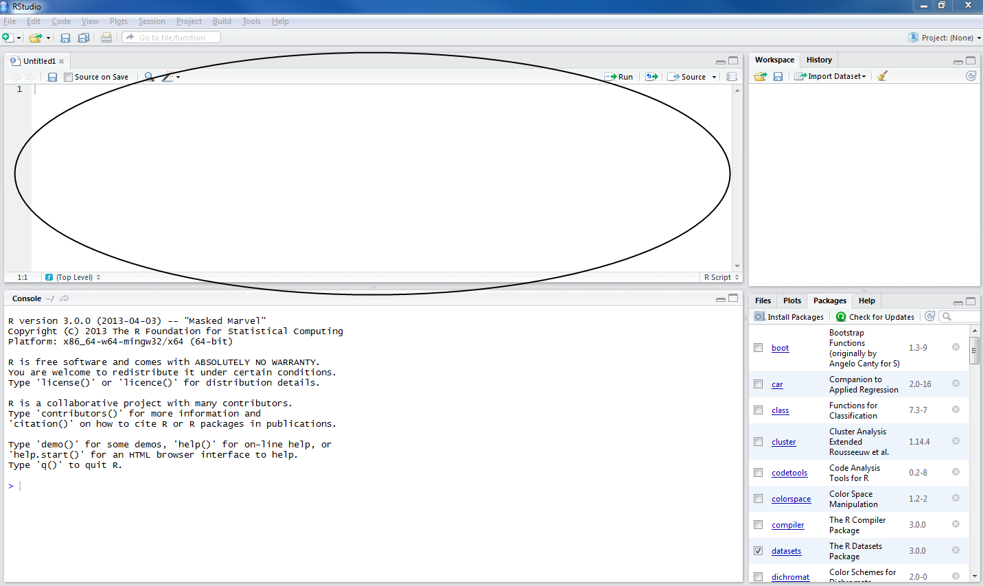
p <- ggplot(mtcars, aes(wt, mpg))
p + geom_point()

— run them and you will see this:

— notice that the plot window, bottom right, shows you a scatterplot.

How did this happen?

Look at the first line of code:

p <- ggplot(mtcars, aes(wt, mpg))

— it creates an object, you can see it listed in the workspace (it was not there before):

— that line of code does a number of things, so I will break it down piece by piece:

p <- ggplot(mtcars, aes(wt, mpg))

p <- ...

— means: create <- (assignment arrow) an object (named p, now in the workspace)

... ggplot( ... )

— means do this using the ggplot() function, which is provided by installing the ggplot2 package then loading (library(ggplot) the ggplot2 package of data and functions

... ggplot(mtcars ...)

— means create the plot using the data in the database (in R: dataframe) called mtcars

— mtcars is a dataframe that gets loaded together with functions like ggplot when you execute: library(ggplot2)

... ggplot( ... aes(wt, mpg))

— aes(wt,mpg) means: map the variables wt and mpg to the aesthetic attributes of the plot.

In the ggplot2 book (Wickham, 2009, e.g. pp 12-), the things you see in a plot, the colour, size and shape of the points in a scatterplot, for example, are aesthetic attributes or visual properties.

— with aes(wt, mpg) we are informing R(ggplot) that the named variables are the ones to be used to create the plot.

Now, what happens next concerns the nature of the plot we want to produce: a scatterplot representing how, for the data we are using, values on one variable relate to values on the other.

A scatterplot represents each observation as a point, positioned according to the value of two variables. As well as a horizontal and a vertical position, each point also has a size, a colour and a shape. These attributes are called aesthetics, and are the properties that can be perceived on the graphic.

(Wickham: ggplot2 book, p.29; emphasis in text)

— The observations in the mtcars database are information about cars, including weight (wt) and miles per gallon (mpg).

[see

http://127.0.0.1:29609/help/library/datasets/html/mtcars.html

in case you’re interested]

— This bit of the code asked the p object to include two attributes: wt and mpg.

— The aesthetics (aes) of the graphic object will be mapped to these variables.

— Nothing is seen yet, though the object now exists, until you run the next line of code.

The next line of code:

p + geom_point()

— adds (+) a layer to the plot, a geometric object: geom

— here we are asking for the addition of geom_point(), a scatterplot of points

— the variables mpg and wt will be mapped to the aesthetics, x-axis and y-axis position, of the scatterplot

The wonderful thing about the ggplot() function is that we can keep adding geoms to modify the plot.

— add a command to the second line of code to show the relationship between wt and mpg for the cars in the mtcars dataframe:

p <- ggplot(mtcars, aes(wt, mpg))
p + geom_point() + geom_smooth()

— here

+ geom_smooth()

adds a loess smoother to the plot, indicating the predicted miles per gallon (mpg) for cars, given the data in mtcars, given a car’s weight (wt).

[If you want to know what loess means – this post looks like a good place to get started.]

Notice that there is an export button on the top of the plots window pane, click on it and export the plot as a pdf.

Where does that pdf get saved to? Good question.

What have we learnt?

— starting a new script

— installing and loading packages

— creating a new plot

Vocabulary

functions

install.packages()

library()

ggplot()

critical terms

object

workspace

package

scatterplot

loess

aesthetics