In the previous post, we revised how to read in dataframes (see also how to read in .csv files as dataframes), using the item norms database as an example (see also here), and we also revised how to get summary information on your dataframe.

We added new understanding by looking at how you can refer to a dataframe variable by name, using the dataframe.name$variable.name notation, which will be useful.

We looked at why as well as how you look at a dataframe – hint: its about making sure your data are in the shape that you think they are.

And, we looked at how you can test for and convert the type of a variable.

In this post, we will be doing all new work on how you refer to elements in a dataframe by place, name or condition.

This will help us to get to the really useful capacity to subset data.

In the next posts, we will look at how you subset a dataframe to help plotting and statistical analysis.

I recommend R-in-Action (Kabacoff, 2011; chapter 4) or the Quick-R website as a companion for this post.

OK, so we have the dataframe item.norms in our workspace, what’s in it?

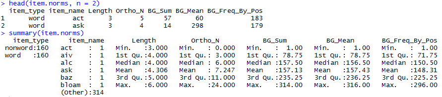
Notice:

— We previously played with converting the BG variables into factor variables then back into numeric variables using as.factor() and as.numeric(). As I am writing the previous post and this post in the same R session, the variables are still being treated as numbers.

— This conversion is not permanent but if you wanted to create a dataframe with the variables converted permanently, I think you would have to output the new dataframe using the write() function, which we will get to.

Referring to elements of a dataframe by place

You can refer to and interact with variables (columns) and observations (rows) and elements (a specific observation or observations in a specific variable or variables) by place, name, or conditionally (by examining a dataframe for if elements meet criteria you set). This is a big area but it is useful to get a flavour now.

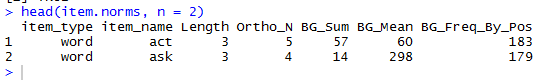
Remember that head() will get you a view of the top rows in a dataframe.

You have seen [] before. In both matrices and dataframes, every element – every cell in a spreadsheet – can be located by the column it is in and the row it is in.

The notation used here is: dataframe[row index, column index]

Dataframe columns and rows are indexed by number:

1- x from left to right among columns;

1 – x from top to bottom among rows.

Let’s try this out using the example item.norms dataframe.

# let's look at the dataframe

head(item.norms, n = 2)

# what is the second variable (column)?

item.norms[, 2]

# what is the second observation (row)?

item.norms[2, ]

# what is the second observation in the second variable?

item.norms[2, 2]

Notice:

— If I am selecting columns, I specify which columns I want but leave the entry blank on rows: [ , which columns].

— If I am selecting rows, I specify which rows I want but leave the entry blank on columns: [which rows, ].

— If you run this code, you will see that “ask” is the entry in the second row of the second column (item names).

— This is not that hard to find out by eye when using excel or SPSS to look at a spreadsheet.

— The use of indices in R becomes extremely useful when you are dealing with larger data sets.

Subsetting dataframes

Let’s take this out for a walk.

I often get datasets where I might want to use only some of the variables (not others) or some of the observations (not others). There are a number of ways I can subset the dataframe.

Subsetting dataframes using the column or row indices

I can select a range of variables or rows by specifying them using the [] notation. I could ask for a set of variables (or observations) by defining a vector of columns (or rows) using the – c(x:y) i.e. from x to y or c(x,y,z) i.e. just x, y and z – notation for creating vectors that we saw earlier here and here. I could delete variables by adding – to the front of column or row indices. I would tend to create a new dataframe from the dataframe I am subsetting, to stay safe.

# I can subset the dataframe using the column or row indices

head(item.norms, n = 2)

# what if I just want the numeric variables?

new.item.norms <- item.norms[, c(3:7)]

head(new.item.norms, n = 2)

# what if I just want the Length and BG_Sum variables?

new.item.norms.2 <- item.norms[, c(3, 5)]

head(new.item.norms.2, n = 2)

# what if I just want the the top ten rows in the dataframe?

new.item.norms.3 <- item.norms[c(1:10),]

head(new.item.norms.3, n = 2)
summary(new.item.norms.3)

# what if I want to get rid of a variable?

# what if I want to get rid of the BG_Mean and item.name variables

new.item.norms.4 <- item.norms[,c(-2, -6)]

head(new.item.norms.4, n = 2)

# use the - operator to get rid of rows also

Notice:

— I might set conditions on

Using the column and row indices is useful.

Generally, however, I tend to prefer selecting variables by name and rows by condition.

Subsetting variables by name

I prefer to subset variables by name because I often deal with dataframes with many (20+) variables and counting the variables to find the right number is both costly and susceptible to error. Better to select variables by name. Obviously, you need to enter the name correctly, so I often copy/paste the name from the output of a head() call in the console into the script window.

Note that in the following I change how I get rid of variables.

# I can subset the dataframe using the column names

head(item.norms, n = 2)

# what if I just want the numeric variables?

new.item.norms.5 <- item.norms[, c("Length", "Ortho_N", "BG_Sum", "BG_Mean", "BG_Freq_By_Pos")]

head(new.item.norms.5, n = 2)

# what if I just want the Length and BG_Sum variables?

new.item.norms.6 <- item.norms[, c("Length", "BG_Sum")]

head(new.item.norms.6, n = 2)

# what if I want to get rid of a variable?

# what if I want to get rid of BG_Mean and item.name variables?

dropvars <- names(item.norms) %in% c("item_name", "BG_Mean")

new.item.norms.7 <- item.norms[!dropvars]

head(new.item.norms.7, n = 2)

Notice:

— In removing variables, I adapted code in R-in-Action (Kabacoff, 2011; p.87):

1. I created a vector of variable names, dropvars, using names(item.norms).

2. names(item.norms) %in% c(“item_name”, “BG_Mean”) created a logical vector with TRUE for each element in names(item.norms) that matched the item_name and BG_Mean variable names, FALSE otherwise.

3. The ! operator reverses those logical values.

4. item.norms[!dropvars] selects columns with TRUE logical values i.e. all except the item_name and BG_Mean variables.

— Pretty nifty, right?

Subsetting observations by condition

I do not usually select observations (rows) by index, I usually subset observations that meet conditions I specify.

# selecting observations by condition

# item.norms holds data on both words and nonwords, what if I want# to focus on just words?

item.norms.words <- item.norms[item.norms$item_type == "word", ]

summary(item.norms)
summary(item.norms.words)

# what if I want to focus on just words of length 3 letters?

item.norms.words.3 <- item.norms[which(item.norms$item_type ==
"word" & item.norms$Length == 3), ]

summary(item.norms)
summary(item.norms.words.3)

Notice:

— In the first example, I am specifying a condition on rows, leaving the entry blank on columns.

— In setting the condition, I am asking R to select those observations that meet the condition that the item_type value is word. This is a logical comparison and I use the logical operator == which means ‘equal to’ or ‘is the same as’.

— What we are doing here is selecting rows according to a logical test: “Is the observation associated with a value on item.norms that is exactly equal to ‘word’? TRUE or FALSE?”

— In R, = means the same as the <- assignment arrow i.e. you are assigning a value to an object name. If all you are doing is asking if something meets a condition (is the same as) then you use ==.

A useful primer on R operators can be found in Quick-R, here.

— In the second example, I am following an example used by Kabacoff (2011; p. 87).

— I am setting two conditions, that there is a subset of just words, and only those words that are three letters in length.

— We break the effect of the code down as follows (see Kabacoff, 2011; p. 87):

1. The logical comparison item.norms$item_type == “word” produces a vector of logic values, TRUE if the observation is about a word, FALSE if it is not: the vector will have as many elements as there are items in item.norms.

2. The logical comparison item.norms$Length == 3 does the same kind of thing, producing a  vector of logical values, TRUE if the item has a length of 3.

3. The & (logical AND) operator combines the two so that a vector is produced if and only if the item is both a word and has a length of 3.

4. The function which() tells us which elements of the joint condition logical vector are TRUE, i.e. indexing where items are words and have length 3.

5. The item.norms[which(…), ] call selects those rows corresponding to the which() index.

Again, this is very neat.

I used to select items in excel by sorting rows but that invited errors (did I sort all the rows?) and was not self-annotating i.e. reproducible, as an operation coded in a .R script is.

I think you can also do this in SPSS but I don’t know because, frankly, doing it in R is easy and safe, so why bother to learn how to do it in SPSS?

How to subset data using the subset() function

I now often use the subset() function to do much of what I have shown in the foregoing.

# selecting variables or observations using the subset() function

head(item.norms, n = 2)

# what if I just want the numeric variables?

new.item.norms.8 <- subset(item.norms, select = c("Length",
"Ortho_N", "BG_Sum", "BG_Mean", "BG_Freq_By_Pos"))

head(new.item.norms.8, n = 2)

# what if I want to get rid of the BG_Mean and item_name variables

new.item.norms.8 <- subset(item.norms, select = -c(BG_Mean,
item_name))

head(new.item.norms.8, n = 2)

# selecting observations by condition using subset()

# item.norms holds data on both words and nonwords, what if I want# to focus on just words?

item.norms.words.4 <- subset(item.norms, item_type == "word")

summary(item.norms)
summary(item.norms.words)

# what if I want to focus on just words of length 3 letters?

item.norms.words.5 <- subset(item.norms, item_type == "word" &
Length == 3)

summary(item.norms)
summary(item.norms.words.5)

As you can see, the syntax involved in using subset() is a bit simpler.

Notice:

— Selecting variables and rows is very easy.

— Using code to do this makes the changes between dataframes reproducible.

— Using this R code is neat, and given its flexibility, powerful.

What have we learnt?

[The code used for this post can be found here.]

We have learnt to refer to elements by row and column indices, using the [,] notation.

We have learnt to select variables by place index, or name.

We have learnt to select observations by place index or condition.

We have learnt how to remove variables or observations.

We have learnt how to use the subset() function to do all these things.

We have also learnt about logical operators.

Key vocabulary

[,]

which()

%in%

:

&

!

–

==

subset()